Systems Foundations for LLMs

Systems Foundations for LLMs

2.1 GPU Architecture - From Silicon to LLM Training

Modern large language models are trained and served almost exclusively on GPUs (Graphics Processing Units). Understanding GPU architecture is essential for making informed decisions about parallelism strategies, memory management, kernel optimization, and infrastructure sizing. This section provides a comprehensive introduction to GPU hardware as it relates to LLM workloads.

2.1.1 Why GPUs for Deep Learning?

GPUs and CPUs represent fundamentally different hardware philosophies. Understanding this difference explains why LLM training is 100-1000× faster on GPUs.

CPUs vs. GPUs - Fundamental Design Philosophy

• CPUs are optimized for latency - they execute a few threads as fast as possible, with large caches, branch predictors, and out-of-order execution. A modern CPU has 8-96 cores.

• GPUs are optimized for throughput - they execute thousands of threads in parallel, each doing simple work. A modern GPU has thousands of "cores" (execution units) grouped into Streaming Multiprocessors (SMs).

Deep learning workloads are dominated by matrix multiplications (O(n3) operations on O(n2) data), which are embarrassingly parallel. A single transformer forward pass for a 70B model requires ∼140 TFLOP of compute per token - perfect for GPU throughput.

2.1.2 NVIDIA GPU Microarchitecture Generations

NVIDIA has released a series of GPU architectures, each bringing key innovations for deep learning:

2.1.3 Common GPUs for LLM Training and Inference

Which GPU to Choose?

• Training 70B+ models: H100/B200 nodes with NVLink (need fast interconnect for tensor parallelism). Minimum 8×H100 per instance.

• Inference (latency-sensitive): H100/H200 for high BW; MI300X for memory-bound (huge KV caches).

• Fine-tuning 7B-13B: A100-80GB is cost-effective. Single GPU with LoRA.

• Budget: A100-40GB or even A10 (24GB) for LoRA on 7B models.

Architecture Year Flagship Key Deep Learning Innovation

Pascal 2016 P100 First HBM GPU; FP16 support; NVLink 1 Volta 2017 V100 Tensor Cores (first generation); mixed-precision training Turing 2018 T4 INT8 inference; RT cores (not for ML) Ampere 2020 A100 BF16 Tensor Cores; TF32; 3rd-gen NVLink; MIG Hopper 2022 H100 FP8 Tensor Cores; TMA; Transformer Engine; NVLink 4 Blackwell 2024 B200 2nd-gen Transformer Engine; NVLink 5 (1.8 TB/s); FP4

Table 2.2: GPU specifications relevant to LLM workloads. All bandwidth figures are bidirectional.

GPU Arch HBM BF16 TF HBM BW NVLink LLM Role

V100-32GB Volta 32 GB 125 TF* 900 GB/s 300 GB/s Legacy; small model fine-tune A100-40GB Ampere 40 GB 312 TF 1.5 TB/s 600 GB/s Budget training/inference A100-80GB Ampere 80 GB 312 TF 2.0 TB/s 600 GB/s Standard RLHF (8-64 for 70B) H100 SXM Hopper 80 GB 990 TF 3.35 TB/s 900 GB/s 3× faster training H200 SXM Hopper 141 GB 990 TF 4.8 TB/s 900 GB/s Fits 70B policy+ref on fewer GPUs B200 SXM Blackwell 192 GB 2250 TF 8.0 TB/s 1800 GB/s Next-gen; 2× over H100

AMD and Google alternatives: MI300X CDNA3 192 GB 1300 TF 5.3 TB/s N/A Most memory; ROCm TPU v5e Google 16 GB 197 TF 1.6 TB/s ICI 1.6 TB/s Cloud-only; JAX/XLA

2.1.4 GPU Internal Architecture - The Streaming Multiprocessor (SM)

A GPU is organized as an array of Streaming Multiprocessors (SMs), each of which is an independent processor with its own register file, shared memory, and execution units. Understanding SMs is key to understanding GPU performance.

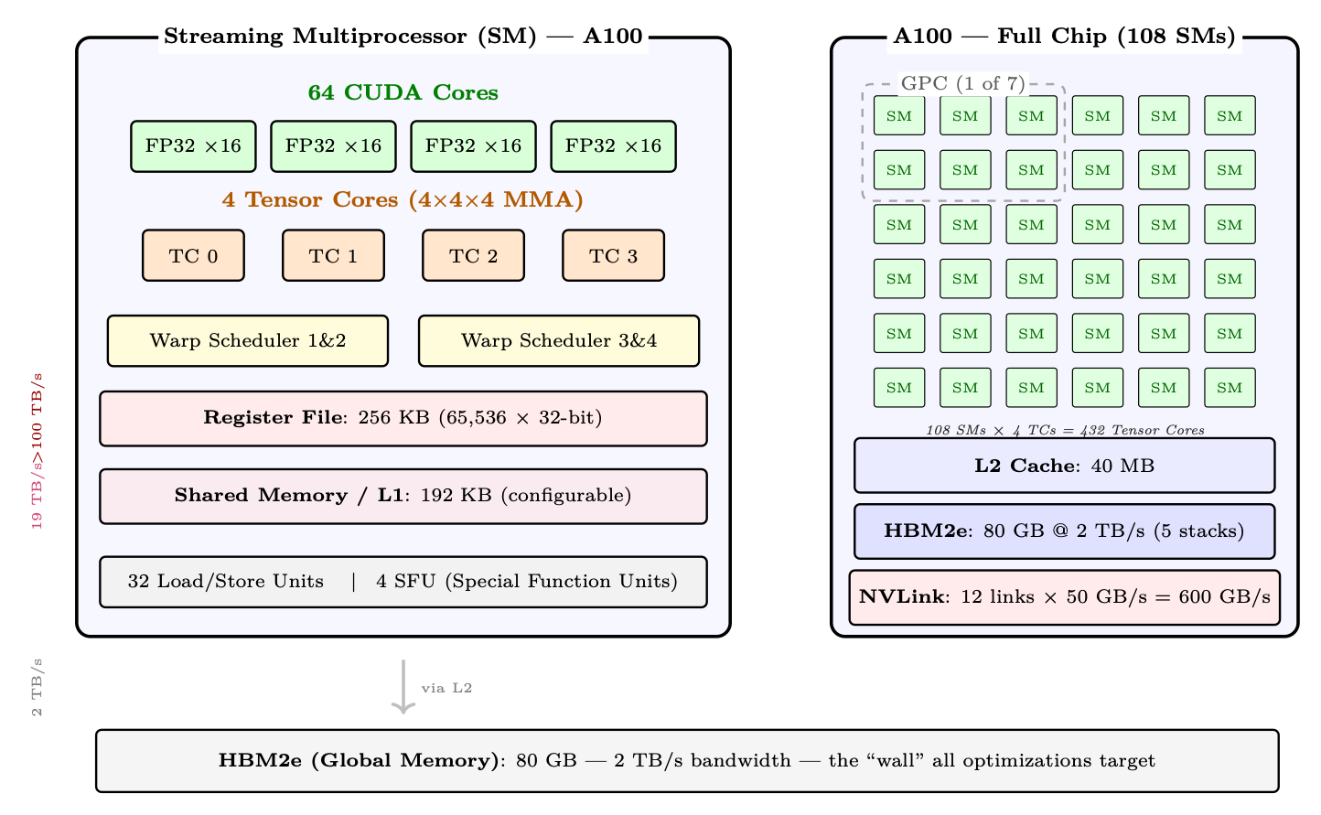
Figure 2.1: Left: Internal structure of a single Streaming Multiprocessor (SM) on A100 -- 64 FP32 CUDA cores, 4 Tensor Cores, 4 warp schedulers, 256 KB register file, and 192 KB shared memory/L1 cache. Right: The full A100 chip contains 108 SMs with shared 40 MB L2 cache and 80 GB HBM2e. Bandwidth annotations (left margin) show the dramatic drop from registers to HBM.

• CUDA Cores: Scalar ALUs for FP32/INT32 operations. 64 per SM on A100. Used for element-wise ops, reductions, and non-matrix operations.

• Tensor Cores: Specialized matrix-multiply-accumulate (MMA) units. Each performs a 4×4×4 fused multiply-add per cycle. 4 per SM on A100, delivering 16× throughput over CUDA cores for supported precisions.

• Register File: Fastest storage (1 cycle latency). Shared among all active threads. Spilling to L1 causes significant slowdown.

• Shared Memory / L1: On-chip SRAM explicitly managed by the programmer. The key to Flash Attention's performance (tiles fit entirely in shared memory).

• Warp Schedulers: Each SM has 4 warp schedulers (A100). A warp = 32 threads executing in lockstep (SIMT model). Schedulers hide memory latency by switching between warps.

The SIMT Execution Model GPUs use Single Instruction, Multiple Threads (SIMT) execution. Within a warp (32 threads), all threads execute the same instruction but on different data. When threads diverge (e.g., if/else), both paths are serialized - called warp divergence. This is why GPU kernels must minimize branching. For LLM workloads, the main operations (GEMM, attention, softmax) have uniform control flow across threads, making them ideal for SIMT execution.

2.1.5 GPU Chip Scaling Across Generations

The evolution of NVIDIA's GPU architectures shows consistent scaling of compute density, on-chip memory, and specialized units for deep learning:

Table 2.3: SM-level scaling across NVIDIA architectures.

Architecture SMs TCs/SM SRAM/SM L2 Key Change

Volta (V100) 80 8 128 KB 6 MB Introduced Tensor Cores Ampere (A100) 108 4 192 KB 40 MB BF16/TF32; larger L2 Hopper (H100) 132 4 256 KB 50 MB TMA; FP8; Thread Block Clusters Blackwell (B200) 148 4 256 KB 128 MB 2× die; FP4; TMEM; NVLink 5

2.1.6 GPU Memory Hierarchy and Bandwidth

Modern GPU training and inference performance is almost entirely determined by how well you manage data movement across the memory hierarchy. Understanding the hierarchy is not optional it is the foundation for every optimization technique discussed in later sections.

GPU Memory Hierarchy - A100 80GB Reference Numbers

Level Capacity Bandwidth Latency Location

Registers ∼256 KB/SM >100 TB/s 1 cycle On-chip, per-thread SRAM (shared) 164 KB/SM ∼19 TB/s ∼20 cy On-chip, per-SM L2 Cache 40 MB total ∼5 TB/s ∼200 cy On-chip, shared HBM2e (VRAM) 80 GB 2 TB/s ∼200 ns On-package (5 stacks) CPU DRAM 512 GB+ ∼25 GB/s ∼10 µs Host (PCIe 4) NVMe SSD TBs 7 GB/s ∼100 µs Host storage

Why the Gaps Are So Large

Each level of the hierarchy is roughly 10× slower and 100-1000× larger than the one above it. The A100 has 312 TFLOP/s of BF16 tensor-core throughput but only 2 TB/s of HBM bandwidth.

Registers. Each CUDA thread has access to a private register file. Registers are the fastest storage on the chip - reads and writes happen in a single clock cycle with no arbitration. The A100 has 65,536 32-bit registers per SM. Spilling registers to local memory (L1/L2) is a major performance hazard.

SRAM - Shared Memory / L1. Each SM has a combined L1/shared memory pool of 192 KB on A100 (256 KB on H100), with up to 164 KB configurable as shared memory on A100. Shared memory is explicitly managed by the programmer (or by the compiler in newer CUDA versions). Flash Attention, for example, is entirely built around the insight that the attention tile computation fits in SRAM.

L2 Cache. The 40 MB L2 on A100 is shared across all 108 SMs. It acts as a staging area between SRAM and HBM. For workloads with good spatial locality (e.g., weight matrices accessed repeatedly across a batch), L2 hit rates can dramatically reduce effective HBM traffic.

HBM - High Bandwidth Memory. HBM is stacked DRAM mounted directly on the GPU package, connected via a wide interposer. The A100 SXM has 80 GB of HBM2e at 2 TB/s. The H100 SXM5 has 80 GB of HBM3 at 3.35 TB/s. This is the primary working memory for model weights, KV caches, activations, and optimizer states.

CPU DRAM via PCIe. Data transfer between GPU HBM and CPU DRAM traverses the PCIe bus. PCIe Gen4 ×16 provides ∼32 GB/s per direction (64 GB/s bidirectional); Gen5 doubles this. This is a ∼60× bandwidth reduction compared to HBM (per-direction). CPU offloading (ZeRO-Infinity, DeepSpeed) exploits this link but must be used carefully to avoid becoming the bottleneck.

NVMe. NVMe SSDs (e.g., Samsung 990 Pro) reach ∼7 GB/s sequential read. ZeRO-Infinity can offload optimizer states to NVMe, but this is only viable when the compute-to-IO ratio is very high (large batch sizes, slow training steps).

2.1.7 Arithmetic Intensity and the Roofline Model

Arithmetic Intensity

I = FLOPs Bytes accessed from HBM (FLOPs / Byte)

A kernel is memory-bound when I < Iridge and compute-bound when I > Iridge, where

Iridge = Peak FLOP/s Peak Bandwidth = 312 × 1012

2 × 1012 = 156 FLOP/Byte (A100 BF16)

Attention Arithmetic Intensity

For a single attention head with sequence length n = 4096, head dim d = 128: FLOPs: QKT costs 2n2d, softmax is O(n2), Attn × V costs 2n2d. Total: ≈4n2d = 4 × 40962 × 128 ≈8.6 GFLOP. Memory traffic (standard, non-Flash implementation):

• Read Q, K: 2 × n × d × 2 = 2 MB

• Write attention scores S = QKT : n2 × 2 = 33.5 MB

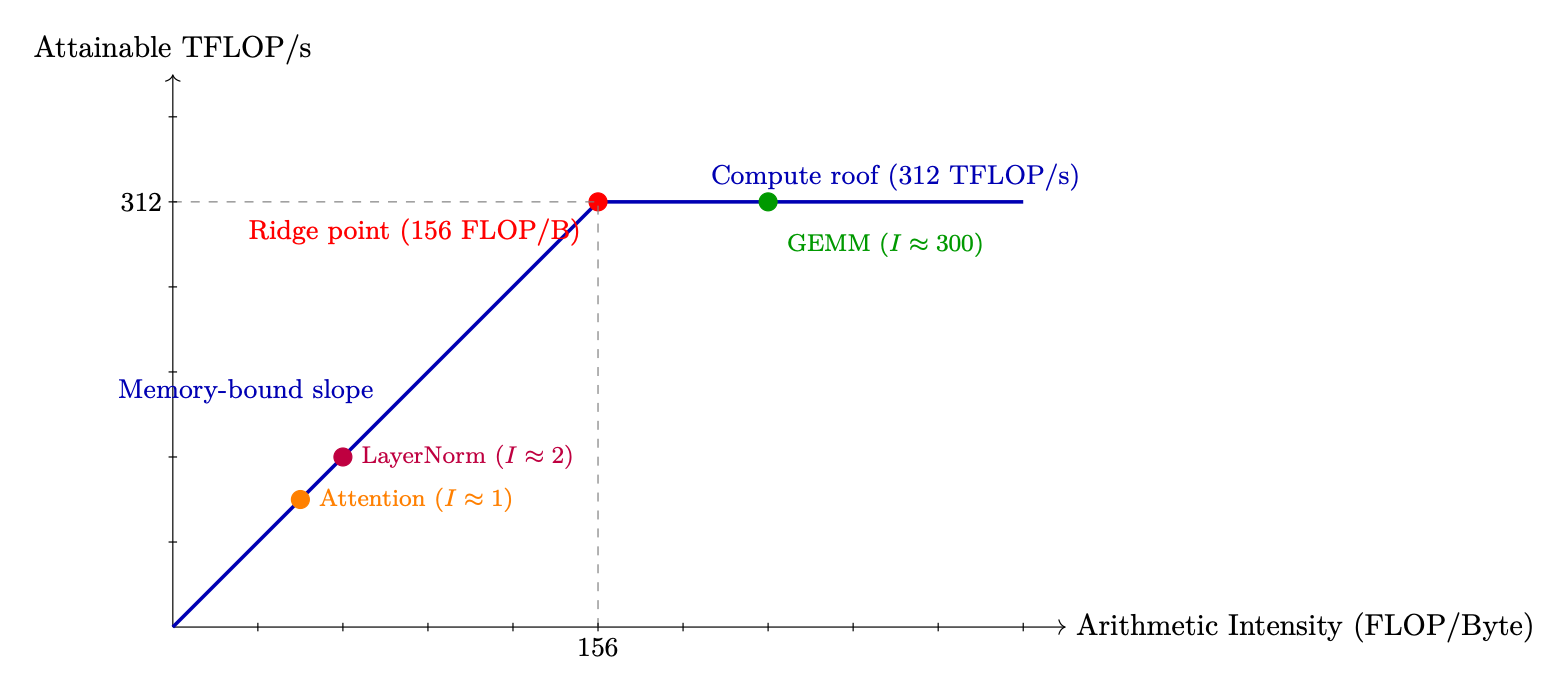
Figure 2.2: Roofline model for A100 BF16. Attention is deep in the memory-bound regime; large GEMMs (FFN layers) are compute-bound.

• Read S for softmax: n2 × 2 = 33.5 MB

• Write softmax output P: n2 × 2 = 33.5 MB

• Read P and V for final matmul: n2 × 2 + n × d × 2 = 34.5 MB

• Write output O: n × d × 2 = 1 MB

Total memory: ≈138 MB (dominated by 4 passes over the n2 attention matrix). Arithmetic intensity:

I = 8.6 × 109

138 × 106 ≈62 FLOP/Byte

This is 62/156 = 40% of the A100 ridge point -- firmly memory-bound. The GPU is 60% idle waiting for memory. Flash Attention fix: By never materializing the n × n matrix (tiling Q, K, V in SRAM), Flash Attention reduces HBM traffic to just reading Q, K, V and writing O: 4 × n × d × 2 = 4 MB. Each byte loaded is reused in O(n) computations (every query attends to every key), so:

I = 4n2d 4 · n · d · 2 = n

2 = 4096

2 = 2048 FLOP/Byte

This is 13× above the ridge point (156) -- deeply compute-bound. The GPU hits its peak 312 TFLOPS, needing only 312T/2048 ≈152 GB/s of bandwidth (7.6% of HBM capacity). Memory is no longer the bottleneck.

2.1.8 Attention is Memory-Bound; FFN is Compute-Bound

Two Regimes in a Transformer

A transformer block has two main components with very different arithmetic intensities:

• Attention: Operates on n × d tensors. The QKT product is O(n2d) FLOPs but requires O(n2) memory for the attention scores. At long sequences, memory traffic dominates attention is memory-bound.

• FFN (MLP): Two large linear layers with weight matrices of shape [dmodel, 4dmodel]. These are large GEMMs with high arithmetic intensity - FFN is compute-bound.

This is why Flash Attention (memory optimization) helps attention but not FFN, while quantization (reducing weight size) helps FFN more than attention.

What Are Tensor Cores? Tensor Cores are specialized matrix-multiply-accumulate (MMA) units introduced in Volta (2017). Each Tensor Core performs a 4 × 4 × 4 matrix multiply in a single clock cycle:

D = A × B + C (4 × 4 matrices)

The A100 has 432 Tensor Cores across 108 SMs (4 per SM, one per sub-partition). At BF16 precision, they deliver 312 TFLOP/s - roughly 16× the throughput of FP32 CUDA cores.

• Supported precisions: FP64, TF32, BF16, FP16, INT8, FP8 (H100+).

• Accumulation: Always in FP32 internally, even for BF16 inputs. This prevents catastrophic cancellation during the dot product.

• Requirement: Tensor Cores are most efficient when matrix dimensions are multiples of 8 (BF16) or 16 (FP8). Padding to these multiples is often worthwhile.

• WGMMA (H100): Hopper introduces warpgroup-level MMA instructions that operate on larger tiles (64×256×16) and can be pipelined with TMA (Tensor Memory Accelerator) data movement.

The Tensor Core Trap

Tensor Cores only help if your kernel is compute-bound. If you are running a small batch (batch size 1, inference), the GEMM tiles are tiny, Tensor Core utilization is low, and you are back in the memory-bound regime. This is why inference engines batch requests aggressively.

2.1.10 Communication Architecture - NVLink, InfiniBand, and PCIe

Distributed LLM training and inference require moving enormous amounts of data between GPUs, nodes, and storage. The communication fabric is often the bottleneck for large-scale training.

PCIe - The Host-Device Link.

PCIe Generations

Generation x16 BW (each dir.) Bidirectional Notes

PCIe Gen3 16 GB/s 32 GB/s Common in older servers PCIe Gen4 32 GB/s 64 GB/s A100 PCIe, most current servers PCIe Gen5 64 GB/s 128 GB/s H100 PCIe, emerging

PCIe is used for:

• CPU ↔GPU data transfers (model loading, CPU offloading)

• Cross-node GPU communication when NVLink is unavailable (rare, very slow)

• NVMe storage access (via CPU)

PCIe is Not for GPU-GPU Communication Never route GPU-GPU communication through PCIe if NVLink is available. PCIe bandwidth (32 GB/s) is 28× lower than NVLink 4 (900 GB/s). In a multi-GPU server without NVLink (e.g., consumer GPUs), inter-GPU bandwidth is limited to PCIe, making tensor parallelism extremely slow.

NVLink Generations

Generation Links Total BW GPU

NVLink 2 6 300 GB/s V100 NVLink 3 12 600 GB/s A100 NVLink 4 18 900 GB/s H100 NVLink 5 18 1800 GB/s B200 (Blackwell)

NVLink is a point-to-point interconnect between GPUs on the same node. Each link is bidirectional. The H100 SXM5 has 18 NVLink 4 links, each providing 50 GB/s bidirectional, for a total of 900 GB/s.

NVSwitch. In DGX H100 systems, all 8 GPUs are connected via NVSwitch - a dedicated switching chip that provides full bisection bandwidth. This means any GPU can communicate with any other GPU at full NVLink speed simultaneously, not just neighbors in a ring.

Ring vs. Full Bisection

In a ring topology (8 GPUs), an AllReduce requires data to travel around the ring. Each link must carry 2(N−1)

N of the total data, so the algorithm bandwidth is Blink × N 2(N−1) (about 0.57×Blink for N = 8). With NVSwitch full bisection, AllReduce can use all links simultaneously with tree-based algorithms, achieving near-peak bandwidth. In practice on DGX H100: ring achieves ∼700 GB/s bus bandwidth, NVSwitch achieves ∼900 GB/s.

InfiniBand - Inter-Node Communication. For communication between nodes (servers), InfiniBand provides high-bandwidth, low-latency networking with direct GPU memory access.

InfiniBand NDR

• NDR 400Gb/s = 50 GB/s per port (unidirectional)

• HDR 200Gb/s = 25 GB/s per port (previous generation)

• RDMA: Remote Direct Memory Access - GPU can read/write remote GPU memory without involving the remote CPU

• GPUDirect RDMA: Data goes directly HBM →NIC →network →NIC →HBM, bypassing CPU and system DRAM entirely

• Latency: ∼1-2 µs for small messages (vs. ∼100 µs for TCP/IP)

Fat-Tree Topology. Large GPU clusters use fat-tree network topologies. A 3-level fat-tree with k-port switches supports k3/4 nodes with full bisection bandwidth. For 400Gb/s NDR switches with k = 64 ports: 643/4 = 65,536 nodes.

Rail-Optimized Topology. In practice, clusters use rail-optimized topologies where each GPU in a node connects to a different top-of-rack switch. This ensures that AllReduce operations (which involve all GPUs) use all network links simultaneously, maximizing bandwidth.

Primitive Use Case Volume

AllReduce Gradient sync (DDP, FSDP) 2(N −1)/N× param size AllGather Collect sharded weights (FSDP) (N −1)/N× param size

ReduceScatter Scatter gradients (FSDP) (N −1)/N× param size AllGather Tensor parallel activation activation size Point-to-Point Pipeline parallel (send/recv) micro-batch activation Broadcast Weight sync (new workers) full model size

Bandwidth Calculation - Gradient AllReduce for 70B Model Setup: 70B parameter model, BF16 gradients, 8 nodes × 8 GPUs = 64 GPUs. Data parallel degree = 64. Gradient size: 70 × 109 × 2 bytes = 140 GB. AllReduce volume per GPU (ring): 2 × (64 −1)/64 × 140 ≈275 GB. Available inter-node bandwidth: 8 GPUs/node × 50 GB/s/GPU = 400 GB/s (with railoptimized topology, all 8 NICs active). AllReduce time: 275/400 ≈0.69 seconds per step. Implication: For a 1-second compute step, communication adds 0.69 seconds (41% of total step time). This is why gradient compression, mixed precision, and FSDP (which overlaps communication with computation) are critical.

Network Topology Diagram. The following diagram illustrates a typical two-node GPU cluster topology showing both intra-node (NVLink) and inter-node (InfiniBand) communication paths.

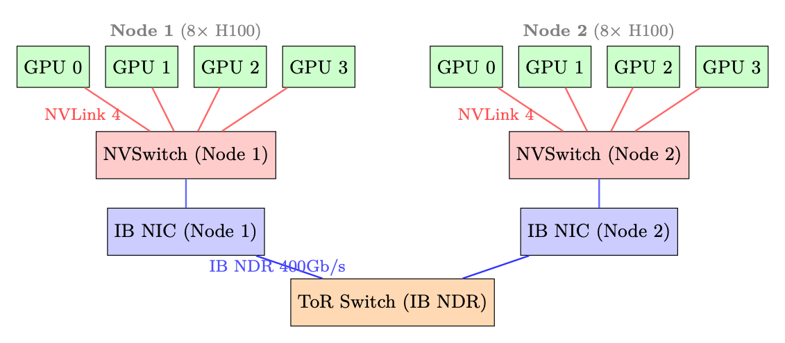
Figure 2.3: Two-node 8-GPU topology. Intra-node: NVLink 4 via NVSwitch (900 GB/s total). Inter-node: InfiniBand NDR 400Gb/s via top-of-rack switch. Each node has 8 IB NICs (one per GPU) for rail-optimized AllReduce.

Choosing Parallelism Based on Bandwidth

• Tensor Parallelism (TP): Requires all-reduce every layer - use only within a node over NVLink. TP=8 is standard for H100 DGX nodes.

• Pipeline Parallelism (PP): Point-to-point between stages - can cross nodes, but adds pipeline bubble overhead. Use when model is too large for TP alone.

• Data Parallelism (DP): AllReduce of gradients - can cross nodes via IB. Scales well with fast IB.

• FSDP/ZeRO: AllGather + ReduceScatter - similar to DP but shards optimizer states. Preferred over DP for large models.

vLLM [157] introduced PagedAttention, which borrows the paging abstraction that operating systems use for RAM and applies it to the GPU's KV cache. During LLM inference, the KV cache - the stored key and value tensors for all previous tokens - is the dominant memory consumer. Managing it efficiently is the central challenge of high-throughput inference.

2.2.1 The KV Cache Fragmentation Problem

KV Cache Memory Formula

For a model with L layers, H heads, head dimension d, and a sequence of n tokens:

KV cache size = 2 × L × H × d × n × bytes_per_element

For Llama-3 70B (BF16): L = 80, H = 8 (GQA), d = 128:

= 2 × 80 × 8 × 128 × n × 2 = 327,680 × n bytes

At n = 4096 tokens: ≈1.3 GB per sequence.

Internal and External Fragmentation

Traditional inference systems pre-allocate a contiguous memory block for each sequence's KV cache, sized to the maximum possible sequence length. This causes two types of waste: Internal fragmentation: A sequence that generates only 500 tokens still holds a block reserved for 4096 tokens. The unused 3596 token slots are wasted. External fragmentation: After many sequences complete, the free memory consists of many small non-contiguous gaps. A new long sequence cannot be allocated even if total free memory is sufficient, because no single contiguous block is large enough. In practice, GPU memory utilization with naive allocation is often only 20-40%.

2.2.2 PagedAttention - Virtual Memory for KV Caches

PagedAttention (Kwon et al., 2023) borrows the paging abstraction from operating systems. Instead of one contiguous block per sequence, the KV cache is carved into fixed-size pages (blocks), and an indirection table--analogous to a CPU page table--translates each sequence's logical token positions into scattered physical GPU memory addresses.

PagedAttention Core Concepts

• Block size: Typically 16 tokens per block (tunable). Each block stores 16 × 2 × L × H × d elements.

• Block table: A per-sequence mapping from logical block index to physical block index in the GPU memory pool.

• Physical block pool: A pre-allocated pool of fixed-size blocks. Allocation is O(1) - just pop from a free list.

• Attention kernel: Modified to gather KV blocks from non-contiguous physical locations using the block table during attention computation.

Block Table Example

Suppose block size = 4 tokens, and we have two sequences:

• Sequence A (7 tokens): logical blocks [0,1] →physical blocks [3, 7]

• Sequence B (5 tokens): logical blocks [0,1] →physical blocks [1, 5]

Physical block 3 holds tokens 0-3 of sequence A. Physical block 7 holds tokens 4-6 of sequence A

2.2.3 Benefits of PagedAttention

Near-zero waste. Internal fragmentation is bounded by at most one partially-filled block per sequence (the last block). With block size 16, worst-case waste is 15 tokens per sequence - negligible. External fragmentation is eliminated because blocks are fixed-size and interchangeable.

Dynamic allocation. Blocks are allocated on demand as the sequence grows. No need to know the final sequence length in advance. This is critical for generation, where output length is unknown.

Prefix sharing (copy-on-write). Multiple sequences sharing a common prefix (e.g., a system prompt) can share the same physical blocks for that prefix. The block table simply points multiple sequences to the same physical blocks. When a sequence needs to write to a shared block (diverging from the prefix), a copy-on-write is triggered.

Prefix Sharing Savings

In a chatbot with a 1000-token system prompt serving 128 concurrent users:

• Without prefix sharing: 128× 1000 × 327,680/109 ≈42 GB just for system prompt KV cache

• With prefix sharing: 1 × 1000 × 327,680/109 ≈0.33 GB

• Savings: ∼128× for the shared prefix portion

Preemption via swap. When GPU memory is exhausted, vLLM can preempt a sequence by swapping its KV blocks to CPU DRAM (or simply discarding them and recomputing later). This is only feasible because blocks are self-contained and non-contiguous - swapping a contiguous allocation would require copying the entire buffer.

2.2.4 Continuous Batching

Traditional batching ("static batching") waits until all sequences in a batch finish before starting new ones. If one sequence generates 500 tokens and another generates 10, the GPU is idle for 490 steps on the short sequence. This is extremely wasteful.

Continuous Batching

Continuous batching (also called iteration-level scheduling) processes one decode step at a time. After each step:

1. Check which sequences have finished (generated EOS token)

2. Remove finished sequences from the batch, freeing their KV blocks

3. Add new waiting sequences to fill the freed slots

4. Run the next decode step with the updated batch

The batch composition changes every step -- sequences join and leave dynamically. This keeps GPU utilization near 100% and dramatically improves throughput (1.5-3× over static batching). PagedAttention is essential here: adding/removing sequences mid-batch requires dynamic KV block allocation/deallocation, which is only efficient with paged memory.

Speculative decoding uses a small draft model (e.g., 1B parameters) to propose k candidate tokens quickly, which the large target model verifies in a single forward pass. All tokens up to the first rejection are accepted (expected acceptance: 3-5 tokens per verification step). This yields 2-3× speedup for latency-sensitive single-sequence generation without any quality loss. vLLM integrates speculative decoding with PagedAttention:

• Draft tokens are allocated speculative KV blocks

• On rejection, speculative blocks are freed (cheap with paged allocation)

• On acceptance, speculative blocks are promoted to the main sequence

• The block table update is O(k) - just updating a few table entries

2.2.6 Concrete Memory Savings - 70B Model at Scale

Memory Budget - 70B BF16 Inference

Setup: Llama-3 70B, BF16, single A100 80GB node (8 GPUs, tensor parallel). Model weights: 70 × 109 × 2 bytes = 140 GB ÷ 8 GPUs = 17.5 GB/GPU. Remaining for KV cache: 80 −17.5 −3 (overhead) = 59.5 GB/GPU. KV cache per token per GPU (with TP=8, each GPU holds 1/8 of heads): 2×80×1×128×2 = 40,960 bytes ≈40 KB/token. Max tokens in KV cache: 59.5 × 109/40,960 ≈1.45 million tokens. With 128 concurrent sequences of 4096 tokens each: 128 × 4096 = 524,288 tokens - well within budget. Without PagedAttention (pre-allocating max length 4096 for each): Same math, but fragmentation wastes ∼50% on average →only 64 sequences fit.

Block Size Tradeoff Larger block sizes reduce the overhead of the block table and improve memory access locality (fewer scattered reads). Smaller block sizes reduce internal fragmentation and enable finer-grained prefix sharing. vLLM defaults to 16 tokens/block, which is a good balance. For very long sequences (100K+ tokens), larger blocks (32-64) may be preferable.

2.2.7 vLLM: End-to-End System

vLLM wraps PagedAttention inside a full serving stack: continuous batching, prefix caching, speculative decoding, and tensor-parallel model sharding all work together to maximize throughput per GPU dollar.

2.2.8 Architecture Overview

2.2.9 Core Components

• API Server: Accepts OpenAI-compatible requests (completions, chat). Tokenizes inputs and creates "sequence groups" (for beam search or multiple samples).

• Scheduler: The brain of vLLM. Maintains three queues:

- waiting: New requests not yet started (prefill pending)

- running: Actively generating tokens (decode phase)

- swapped: Preempted requests whose KV cache was offloaded to CPU

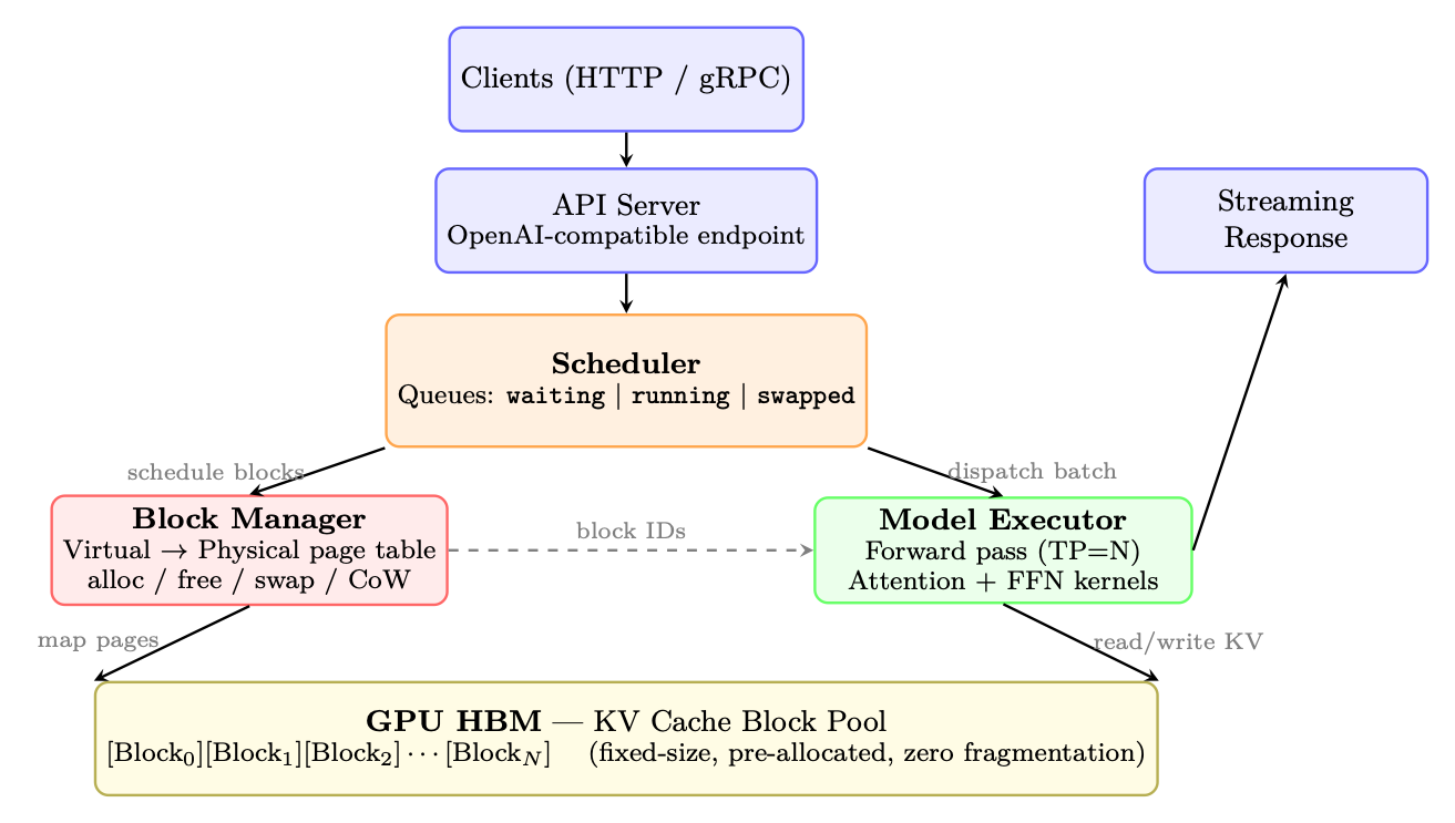
Figure 2.4: vLLM architecture: Requests flow top-down. The Scheduler manages admission and preemption, the Block Manager handles virtual-to-physical KV cache mapping (like OS page tables), and the Model Executor runs batched inference reading from the pre-allocated block pool in GPU HBM.

• Block Manager: Implements the virtual memory abstraction for KV caches. Maps logical blocks (per-sequence) to physical blocks (in GPU memory pool). Handles:

- Allocation (new tokens generated →new blocks needed)

- Copy-on-write (for beam search: multiple beams share prefix blocks, copy only on divergence)

- Swap (GPU ↔CPU migration when preempting/resuming)

- Prefix caching (reuse cached blocks when prompts share common prefixes)

• Model Executor: Runs the actual LLM forward pass. Manages tensor parallelism across GPUs, dispatches attention kernels that read from paged KV cache blocks.

• KV Cache Pool: Pre-allocated GPU memory divided into fixed-size blocks (default: 16 tokens × num_heads × head_dim × 2 bytes per block). No dynamic allocation at runtime → zero fragmentation.

2.2.10 Request Lifecycle (End-to-End Flow)

1. Arrival: Client sends prompt. API server tokenizes it, creates a SequenceGroup, places it in the waiting queue.

2. Scheduling: At each step, the scheduler runs:

(a) Check if any swapped sequences can be resumed (enough free blocks).

(b) Check if any waiting sequences can start prefill (enough blocks for the full prompt).

(c) Budget remaining blocks across running sequences (need 1 new block per sequence per step if current block is full).

(d) If over budget: preempt lowest-priority running sequences (swap KV to CPU or recompute later).

5. Block Allocation: After each decode step, if the last block for a sequence is full, the Block Manager allocates a new physical block and maps it to the next logical block.

6. Completion: When a sequence hits EOS or max length, it's removed from running. Its physical blocks are freed immediately →available for other sequences. Response is streamed back to client.

2.2.11 Prefix Caching (Automatic Prompt Caching)

When multiple requests share a common prefix (system prompt, few-shot examples):

1. Hash the token content of each logical block.

2. On new request arrival, check if any prefix blocks are already in the cache.

3. If hit: skip prefill for those tokens, directly reuse physical KV blocks. Time-to-first-token drops dramatically.

4. Eviction: LRU policy. Cached blocks are freed only when memory pressure requires it.

Impact: For chat applications with long system prompts (2K+ tokens shared across all users), prefix caching reduces TTFT by 60-80%.

2.2.12 Guided (Constrained) Decoding in vLLM

vLLM natively supports constrained decoding (Section 1.12.11) through pluggable backends, enabling guaranteed structured output at serving time with minimal performance overhead.

Supported constraint types. The OpenAI-compatible API accepts constraints via the guided_* parameters or the response_format field:

from openai import OpenAI client = OpenAI(base_url="http :// localhost :8000/ v1")

# --- JSON Schema constraint --- response = client.chat.completions.create(

model="meta -llama/Llama -3-70B-Instruct", messages =[{"role": "user",

"content": "Extract: name , age , city from: "

"'John is 30 and lives in NYC'"}], extra_body ={

"guided_json": {

"type": "object", "properties": {

"name": {"type": "string"}, "age": {"type": "integer"}, "city": {"type": "string"} }, "required": ["name", "age", "city"] } } ) # Output is guaranteed valid JSON matching the schema

# --- Regex constraint --- response = client.completions.create(

"guided_regex": r"\d{1 ,3}\.\d{1 ,3}\.\d{1 ,3}\.\d{1 ,3}" } )

# --- Choice constraint --- response = client.completions.create(

model="meta -llama/Llama -3-70B-Instruct", prompt="Sentiment: ", extra_body ={"guided_choice": ["positive", "negative", "neutral"]} )

Backend architecture. vLLM delegates mask computation to a backend engine:

• XGrammar (default since v0.7): Pushdown-automaton engine supporting JSON schemas, regexes, and arbitrary EBNF grammars. Fastest for complex schemas due to efficient C++ core.

• Outlines [115]: FSM-based; supports JSON and regex. Used as fallback when XGrammar is unavailable.

The mask is applied after the model's forward pass produces logits and before sampling--adding <1 ms per step in practice, since the FSM/PDA state transition and precomputed index lookup are O(1).

Performance impact. Because the constraint only masks logits (no recomputation of attention or FFN), throughput loss is negligible (<2% in benchmarks). The main cost is compilation of the schema into an FSM/PDA index, which takes 0.5-5 s depending on schema complexity. vLLM caches compiled schemas across requests, so this cost is paid once per unique schema.

Structured Output ̸= Correct Output

Constrained decoding guarantees the output is syntactically valid (parses as JSON, matches the schema types). It does not guarantee semantic correctness--the model may still hallucinate values that parse correctly but are factually wrong. Always validate business logic downstream.

Table 2.4: vLLM performance vs. alternatives (70B model, A100 × 4, TP=4).

Metric vLLM HF Generate Why

Throughput (tok/s) 2,500-4,000 300-600 Continuous batching + PagedAttention Memory utilization 90-95% 50-60% Zero fragmentation, dynamic block alloc Max concurrent seqs 200-500 16-32 Paged KV eliminates per-seq reservation Time-to-first-token 100-300ms 500-2000ms Prefix caching for repeated system prompts

Chapter 3