LLM Architecture and Optimization Methods

LLM Architecture and Optimization Methods

This section covers the foundational architecture of large language models and the key optimization techniques that make training and inference efficient. Topics are ordered as a curriculum: we begin with the transformer itself, then cover how to train it efficiently, how to adapt it cheaply, how to compress it, how to scale it, and how to accelerate its inference.

1.1 How LLMs Work: An Intuitive Overview

Before diving into architectural details, let us build intuition for how a large language model transforms text into text. The entire process follows a simple pipeline: text →tokens →representations → tokens →text.

Embedding Layer

Transformer Layers (×L)

Vocab Logits Decode Output Text

Raw Text Tokenizer Token IDs

autoregressive loop (append token to input)

Figure 1.1: The LLM pipeline: text is tokenized into subword units, converted to integer IDs, embedded as dense vectors, processed through transformer layers, projected to vocabulary logits, and decoded back to text. The dashed loop shows autoregressive generation--each output token is appended to the input for the next forward pass.

The Four Key Stages

1. Tokenization: Raw text is split into subword pieces (not characters, not full words) using a learned vocabulary. "unhappiness" might become ["un", "happiness"] or ["unhapp", "iness"].

2. Embedding: Each token ID indexes into a learned embedding table, producing a dense vector in Rd (typically d = 4096). These vectors capture semantic meaning--similar words get similar vectors.

3. Contextual Processing: The transformer stack processes all embeddings in parallel, using self-attention to let each position "read" from all other positions. After L layers, each position's hidden state encodes rich contextual information.

4. Prediction: The final hidden state is projected to a probability distribution over the full vocabulary, and a decoding strategy selects the next token.

1.2 Tokenization

Character-level models need very long sequences (expensive attention). Word-level models cannot handle rare or novel words. Subword tokenization strikes the ideal balance: common words are single tokens ("the" →[the]), rare words decompose into known pieces ("cryptocurrency" → ["crypt", "ocur", "rency"]), and the vocabulary stays manageable (32K-128K tokens).

1.2.1 Why Not Characters or Words?

Table 1.1: Trade-offs of different tokenization granularities.

Granularity Vocab Size Seq Length Issues

Character ∼256 Very long Attention cost O(n2); hard to learn long-range semantics Word ∼500K+ Short Cannot handle rare/novel words; huge embedding table Subword 32K-128K Moderate Best trade-off: short sequences, open vocabulary

1.2.2 Byte-Pair Encoding (BPE)

BPE [24] is the dominant tokenization algorithm used by GPT, Llama, Mistral, and most modern LLMs.

BPE Algorithm

1. Start with a vocabulary of individual characters (bytes)

2. Count all adjacent symbol pairs in the training corpus

3. Merge the most frequent pair into a new symbol

4. Repeat steps 2-3 for k iterations (until desired vocabulary size)

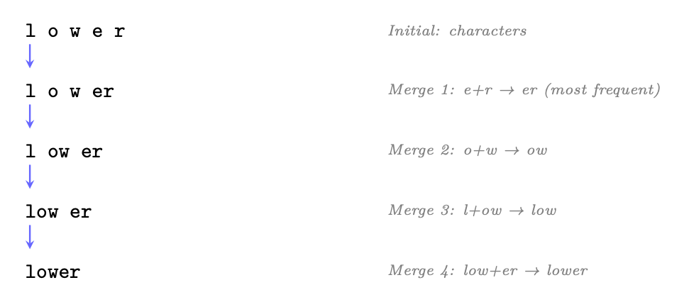
Figure 1.2: BPE tokenization example: starting from characters, the algorithm iteratively merges the most frequent adjacent pairs until the word becomes a single token or the vocabulary budget is exhausted.

Table 1.2: Comparison of subword tokenization algorithms.

Method Used By Key Idea

BPE GPT-4 [23], Llama3 [25], Mistral [26] Bottom-up merging of frequent pairs; deterministic WordPiece BERT [27], DistilBERT [28] Similar to BPE but maximizes likelihood of training data Unigram LM SentencePiece (T5 [29], XLNet [30]) Top-down: start with large vocab, prune by likelihood impact Byte-level BPE GPT-2 [31]+ BPE on raw bytes (no unknown tokens possible); 256 base vocab

1.2.4 Tokenization Best Practices

1. Vocabulary size matters: 32K is minimal; 128K enables better multilingual coverage and code handling. Llama-3 uses 128K tokens.

2. Special tokens: Always include <bos>, <eos>, <pad>, <unk>. For instruction-tuned models, add role markers (<|user|>, <|assistant|>).

3. Fertility: Measure tokens-per-word across languages. High fertility (many tokens per word) indicates poor coverage for that language.

4. Never tokenize across boundaries: Spaces, punctuation, and digits should be handled consistently. Most modern tokenizers prepend a space marker ("the") to distinguish word-initial vs. continuation tokens.

5. Numbers: Consider digit-level tokenization for arithmetic tasks. "2024" as ["2","0","2","4"] enables digit-by-digit reasoning.

6. Code: Ensure whitespace (indentation) is tokenized efficiently. Llama-3 tokenizes runs of spaces as single tokens.

1.2.5 Tokenization in Practice: HuggingFace Example

The transformers library provides a unified interface for all tokenizers. The following demonstrates encoding and decoding with a modern LLM tokenizer:

from transformers import AutoTokenizer

# Load Llama -3 tokenizer (128K vocabulary , byte -level BPE) tokenizer = AutoTokenizer. from_pretrained ("meta -llama/Meta -Llama -3-8B")

text = " Reinforcement learning optimizes long -term rewards."

# Encode: text -> token IDs token_ids = tokenizer.encode(text) print(token_ids) # [128000 , 29934 , 262, 11008 , 4815 , 6900 , 1317 , 9860 , 21845 , 13]

# Decode individual tokens to see subword splits tokens = tokenizer. convert_ids_to_tokens (token_ids) print(tokens) # ['<| begin_of_text|>', 'Re ', 'inforce ', 'ment ', ' learning ', # ' optimizes ', ' long ', '-term ', ' rewards ', '.']

# Tokenize with attention mask (for batched inputs with padding) batch = tokenizer(

["Short text.", "A much longer input sentence for comparison."], padding=True , return_tensors ="pt" ) print(batch.keys ()) # dict_keys ([' input_ids ', 'attention_mask '])

Listing 1.1: Tokenization encode/decode with HuggingFace Transformers.

1.2.6 Special Tokens and Structured Prompts

Special tokens are reserved vocabulary entries that carry structural meaning rather than linguistic content. They are critical for controlling model behavior.

Table 1.3: Common special tokens across LLM families.

Token Alias Purpose

<bos> / <|begin_of_text|> BOS Marks start of sequence <eos> / <|end_of_text|> EOS Marks end of sequence; stops generation <|user|> -- Marks start of user turn in chat <|assistant|> -- Marks start of assistant turn in chat <pad> PAD Fills batch to uniform length; masked in attention <unk> UNK Out-of-vocabulary placeholder (rare with BPE) [SEP] SEP Separates segments (BERT-style) [CLS] CLS Classification token (BERT) [MASK] MASK Masked token for MLM pretraining

Role Markers for Instruction-Tuned Models. Modern chat models use special tokens to delineate conversational structure. These are not trained to carry semantic meaning--they are structural delimiters that the model learns to parse:

# Llama -3 chat template messages = [

{"role": "system", "content": "You are a helpful assistant."}, {"role": "user", "content": "Explain PPO in one sentence."}, ]

# apply_chat_template handles all special token insertion prompt = tokenizer. apply_chat_template (messages , tokenize=False) print(prompt) # <| begin_of_text |><| start_header_id |>system <| end_header_id |> # # You are a helpful assistant .<| eot_id |><| start_header_id |>user <| end_header_id |> # # Explain PPO in one sentence .<| eot_id |><| start_header_id |>assistant <| end_header_id|> # #

Listing 1.2: Chat template with special tokens (Llama-3 format).

Special Token Best Practices

• Never split special tokens: They must be atomic--ensure your tokenizer treats them as single units, not character sequences.

• Mask loss on special tokens: During SFT, do not compute loss on structural tokens (role markers, separators). The model should not "learn" to predict formatting.

• Tool/function calling: Define dedicated tokens like <|function|>, <|result|> to create unambiguous boundaries between reasoning and action.

• Consistent handling in RL: During PPO/GRPO, ensure the reference model and policy model use identical tokenization and special token handling--mismatches corrupt KL computation.

• EOS handling: During generation, ensure EOS is included in the action space. If the model cannot emit EOS, responses grow unbounded (common RL failure mode).

1.3 The Transformer Architecture

The Transformer [6] is the foundation of all modern LLMs. Understanding its components is essential for grasping every optimization and training method in this guide.

1.3.1 High-Level Structure

A decoder-only transformer processes tokens sequentially through embedding, repeated attention+FFN blocks, and a final projection to vocabulary logits. Figure 1.3 shows the complete architecture.

1.3.2 The Original Encoder-Decoder Transformer

The Transformer was originally introduced [6] as an encoder-decoder architecture for sequenceto-sequence tasks (machine translation, summarization). While modern LLMs predominantly use decoder-only variants (GPT-style), understanding the full architecture is essential because crossattention and masked self-attention -- both originating here -- remain fundamental building blocks.

Encoder. The encoder processes the entire input sequence bidirectionally -- each token attends to all other tokens (no causal mask). This produces a rich contextual representation Henc ∈Rn×d

where each position encodes information about the full input:

• Input: Token embeddings + sinusoidal positional encodings

• Each layer: Multi-Head Self-Attention →Add & Norm →FFN →Add & Norm

• No causal mask: Position i attends to all positions 1, . . . , n

• Output: Contextual representations of the full input sequence

Decoder -- Masked Multi-Head Self-Attention. The decoder generates output tokens one at a time (autoregressively). To prevent the model from "seeing the future," the self-attention in the decoder uses a causal mask:

QKT

!

√dk + M

MaskedAttn(Q, K, V ) = softmax

V (1.1)

where the mask M is:

( 0 if i ≥j (can attend) −∞ if i < j (future token -- blocked)

Mij =

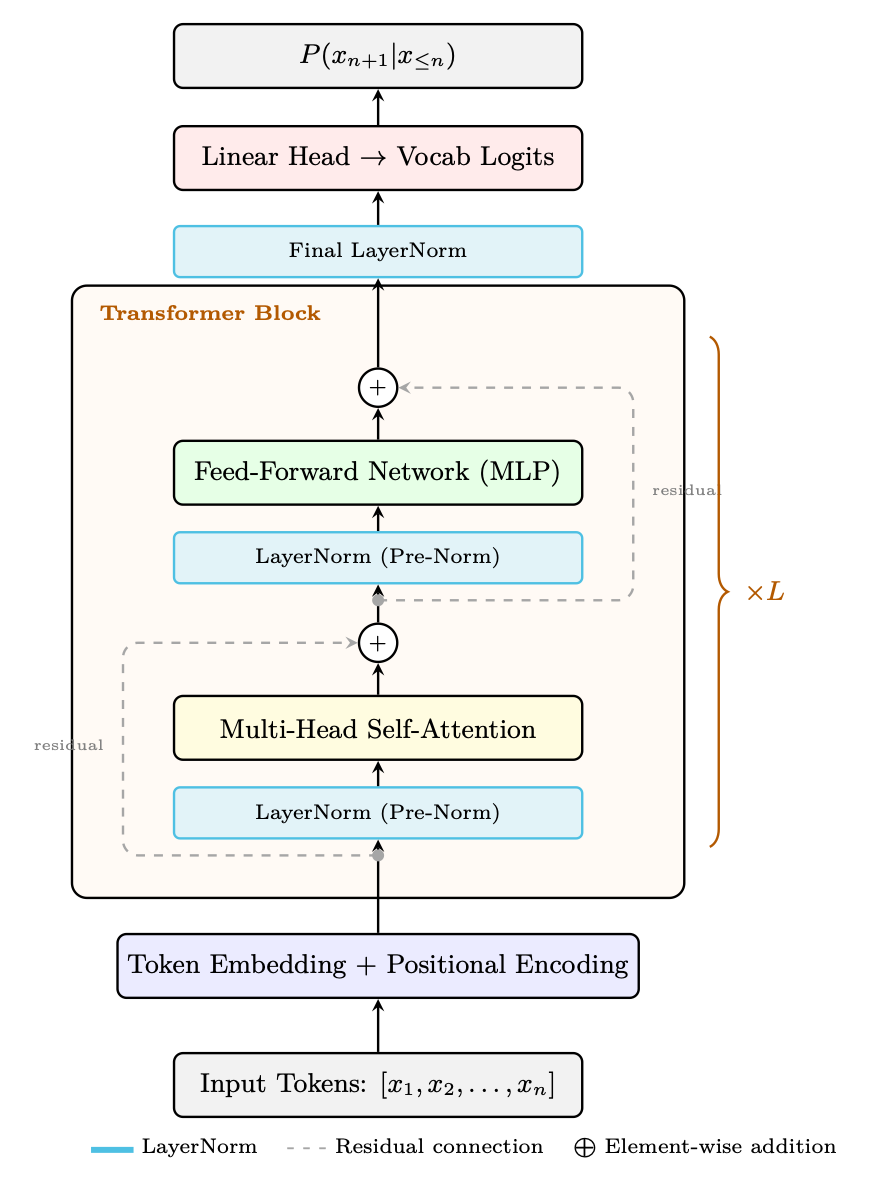
Figure 1.3: Decoder-only Transformer block (GPT-style, Pre-Norm variant). Each sub-layer (attention, FFN) is preceded by LayerNorm and followed by a residual addition: x + SubLayer(LN(x)). This Pre-Norm ordering (used by Llama, GPT-3, Mistral) stabilizes training without warmup, unlike the original Post-Norm (which applies LayerNorm after the addition). L identical blocks are stacked, followed by a final LayerNorm and linear projection to vocabulary logits.

Why Masking Matters

During training, the decoder processes the entire target sequence in parallel (teacher forcing), but each position must only attend to previous positions to maintain the autoregressive property. The mask ensures that generating token t uses only information from tokens 1, . . . , t−1. At inference, tokens are generated one-by-one so the mask is implicit -- but during training it enables parallel computation while preserving causality.

Decoder -- Cross-Attention. After masked self-attention, each decoder layer applies crossattention where the decoder attends to the encoder's output representations. This is the mechanism by which the decoder "reads" the input:

QdecKT enc √dk

!

CrossAttn(Qdec, Kenc, Venc) = softmax

Venc (1.2)

• Queries come from the decoder's previous sublayer (the masked self-attention output)

• Keys and Values come from the encoder's final output Henc

• No mask is applied -- every decoder position can attend to every encoder position

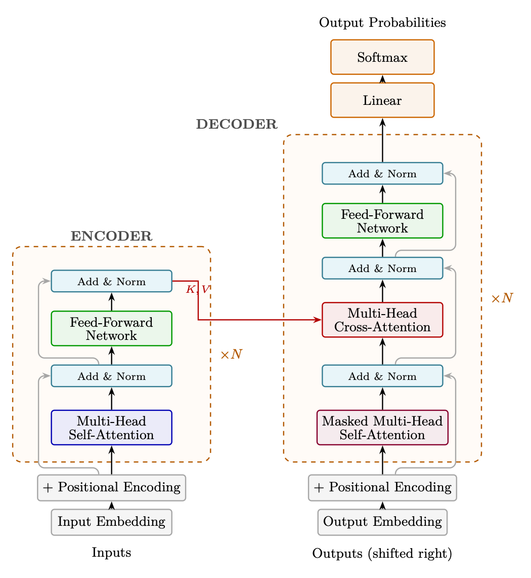
Figure 1.4: The original Transformer architecture (Vaswani et al., 2017). The encoder (left) processes the full input with bidirectional self-attention. The decoder (right) generates tokens autoregressively using masked self-attention and cross-attention to encoder representations. Dashed boxes indicate the repeated layer block (×N); gray lines show residual connections bypassing each sub-layer. Note: the original work uses Post-Norm (LayerNorm applied after the residual addition: LN(x + SubLayer(x))), unlike modern LLMs which use Pre-Norm.

Full Decoder Layer. Each decoder layer contains three sublayers (vs. two in the encoder):

1. Masked Multi-Head Self-Attention + Residual + LayerNorm

2. Multi-Head Cross-Attention (to encoder output) + Residual + LayerNorm

3. Feed-Forward Network + Residual + LayerNorm

Modern LLMs almost exclusively use decoder-only architectures, but understanding the trade-offs with encoder-decoder designs clarifies why.

Architecture Examples Use Case

Decoder-only GPT-4 [23], Llama [25], Mistral [26], Qwen [32] Autoregressive generation; dominant for chat/reasoning Encoder-decoder T5 [29], BART [33], FlanT5 [34] Seq2seq (translation, summarization); less common now Encoder-only BERT [27], RoBERTa [35] Classification/embeddings; not for generation

Why Decoder-Only Won

Decoder-only models are simpler (one model, one loss), scale better (all parameters contribute to generation), and support unified training (pretraining = next-token prediction = fine-tuning objective). Encoder-decoder models waste capacity on the encoder for pure generation tasks.

1.3.4 Embeddings: From Discrete Tokens to Continuous Space

Before any attention or computation happens, the transformer must convert discrete token IDs into continuous vectors that neural networks can process. This is the role of the embedding layer.

What is an Embedding? An embedding is a learned dense vector representation of a discrete symbol. Instead of representing the word "king" as a one-hot vector of size |V| = 128,000 (mostly zeros), we represent it as a compact vector in Rd (e.g., d = 4096) that captures its meaning. The key insight: similar concepts get nearby vectors. In a well-trained embedding space:

• "king" and "queen" are close (both royalty)

• "king" and "bicycle" are far apart (unrelated)

• Vector arithmetic captures relationships: ⃗ king − ⃗ man + ⃗ woman ≈ ⃗ queen

The Embedding Table. In practice, the embedding layer is simply a matrix E ∈R|V|×d where row i stores the embedding vector for token i:

embed(xt) = E[xt] ∈Rd (1.3)

For a sequence of token IDs [x1, x2, . . . , xn], embedding is a simple table lookup (indexing operation): H0 = [E[x1]; E[x2]; . . . ; E[xn]] ∈Rn×d

Embedding Table in Transformers

• Size: |V| × d. For Llama-3: 128,256 × 4,096 = 525M parameters (6.5% of 8B model).

• Initialization: Random (Xavier/normal), then learned via backpropagation.

• Weight tying: Many models share the embedding matrix with the output projection head: Whead = ET . This saves parameters and creates a symmetric encode-decode structure.

• Input: Token ID (integer) →Output: Dense vector in Rd.

• Gradient flow: During training, only the rows corresponding to tokens in the current batch receive gradient updates (sparse update).

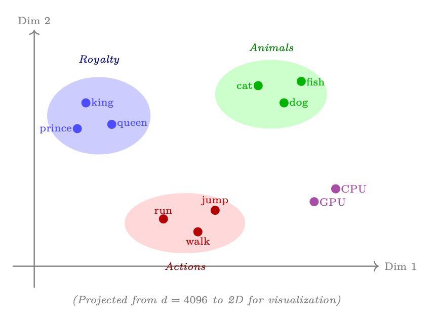
Figure 1.5: Embedding space visualization (2D projection): semantically similar words cluster together. The embedding table learns these positions during pretraining, capturing meaning purely from co-occurrence patterns in text.

Why Embeddings Work

The embedding table is learned end-to-end with the rest of the model. Because the model is trained to predict the next token, it must learn representations where tokens that appear in similar contexts get similar vectors. This is the distributional hypothesis: "you shall know a word by the company it keeps" [36]. The embedding layer compresses this statistical structure into dense geometry.

The Anisotropy Problem. A critical issue arises when using pretrained embeddings (e.g., from BERT or GPT-2) for downstream tasks like retrieval (RAG) or bootstrapping recommender systems: the learned representations are highly anisotropic--they occupy a narrow cone in the embedding space rather than being uniformly distributed across all directions [37]. Why this matters for applications:

• RAG / Retrieval: If all embeddings have cosine similarity > 0.7 regardless of content, retrieval rankings become nearly random--the system cannot distinguish relevant from irrelevant passages.

• Recommender systems: Using pretrained LLM embeddings to represent items/users only works if the geometry preserves meaningful similarity structure.

• Clustering: Anisotropic embeddings collapse clusters, making it impossible to discover natural groupings.

Resolution: Whitening. A simple and effective fix is whitening [38]--a linear transformation that makes the embedding distribution isotropic (zero mean, identity covariance):

˜h = D−1/2UT (h −µ) (1.4)

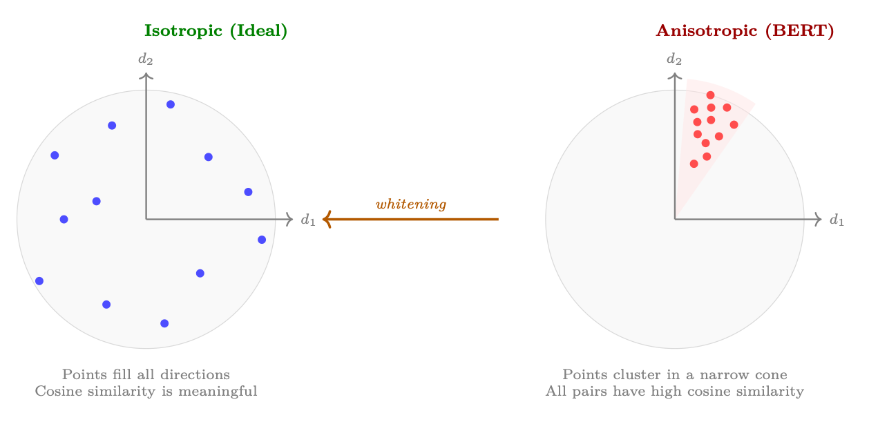
Figure 1.6: Isotropy vs. anisotropy in embedding spaces. Left: isotropic embeddings spread uniformly, making cosine similarity a reliable measure of semantic relatedness. Right: anisotropic embeddings (as found in BERT) cluster in a narrow cone, causing all pairs to have high cosine similarity regardless of semantic content. Whitening transforms the space to restore isotropy.

Whitening in Practice

• What it does: Rotates and scales the embedding space so all directions have equal variance (unit covariance).

• Effect: Cosine similarity becomes meaningful--semantically similar pairs score high, dissimilar pairs score low.

• Bonus: Can simultaneously reduce dimensionality by keeping only the top-k eigenvectors (similar to PCA), making retrieval faster.

• Cost: Requires computing the covariance matrix over a representative corpus (one-time, O(N · d2)). The transform itself is a simple matrix multiply at inference.

• Alternative approaches: Contrastive fine-tuning (SimCSE), flow-based normalization, or training with isotropy-promoting regularizers.

1.3.5 Self-Attention Mechanism

Self-attention is the core operation that allows each token to attend to every other token in the sequence, computing a weighted combination based on relevance.

Scaled Dot-Product Attention

Given input sequence X ∈Rn×d, we compute:

Q = XWQ, K = XWK, V = XWV (WQ, WK, WV ∈Rd×dk)

QKT

!

√dk + M

Attention(Q, K, V ) = softmax

V

where M is the causal mask (for autoregressive models): Mij = 0 if i ≥j, else −∞. Intuition: Each token "attends" to all previous tokens, computing a weighted average of their values based on query-key similarity.

Computational Complexity. The naive attention computation has quadratic cost in sequence length:

For a 128K-token context with d = 4096, the attention matrix alone is 128K × 128K = 16.4 billion entries (64 GB in FP32). This quadratic scaling is the fundamental bottleneck for long-context LLMs.

Table 1.4: Attention cost scaling: why naive implementation is prohibitive for long sequences.

Seq Length Attention Ops Matrix Size Practical Impact

2K 4M 16 MB Fast; fits in SRAM 8K 64M 256 MB Manageable with FlashAttention 32K 1B 4 GB Requires memory-efficient kernels 128K 16B 64 GB Exceeds single GPU HBM 1M 1T 4 TB Impossible without sub-quadratic methods

Approaches to Taming Attention Cost. Several families of solutions address this quadratic bottleneck:

1. Exact attention with IO-awareness (FlashAttention [7]): Does not reduce computational complexity but eliminates the need to materialize the n × n matrix in HBM by computing attention in tiles that fit in SRAM. Crucially, FlashAttention is orthogonal to the sparse patterns below--it is an execution engine, not an attention pattern. Production systems routinely combine FlashAttention with sliding windows or block-sparse masks, getting both IO efficiency and reduced FLOPs. We cover the algorithm in detail in Section 1.6.

2. Sliding window / local attention: Each token only attends to the w nearest tokens (e.g., w = 4096). Cost becomes O(n · w)--linear in n. Used by Mistral [26] (window = 4096) and Longformer [39]. Trades global context for efficiency; works well because most attention is local in practice. In modern stacks, the sliding-window mask is executed inside a FlashAttention kernel.

3. Sparse attention patterns: Combine local windows with periodic global tokens (e.g., every 512th token attends to all). BigBird [40] and LongT5 [41] use this. Preserves some long-range connectivity at O(n√n) cost. Again, FlashAttention serves as the underlying kernel for the non-zero attention blocks.

4. Linear attention / state-space models: Replace softmax(QKT )V with ϕ(Q)(ϕ(K)T V ) using associativity, or reformulate as a recurrence (Mamba [42], RWKV [43]). Theoretically O(n · d2) total. Unlike approaches 2-3 above, these are architectural replacements that alter model expressiveness--softmax-free attention is fundamentally less expressive, and empirically these models still lag behind transformers on tasks requiring precise long-range retrieval or complex reasoning.

5. KV cache compression: At inference, compress or evict old KV pairs to bound memory. Techniques include: H2O [44] (heavy-hitter oracle--keep only high-attention keys), StreamingLLM [45] (keep initial "attention sink" tokens + recent window), and quantized KV caches [46].

FlashAttention + Sparse Patterns = Best of Both Worlds

A common misconception is that FlashAttention is an alternative to sparse attention. It is not--it is an IO optimization for the attention kernel that composes freely with any attention mask. Modern production systems (e.g., Mistral, DeepSeek) use FlashAttention as the execution engine underneath a sliding-window or block-sparse mask. This gives you both reduced FLOPs (from sparsity) and optimal memory access patterns (from tiling). RingAttention [47] extends this further to multi-device settings, distributing the tiled computation across GPUs along the sequence

1.3.6 Multi-Head Attention

Rather than computing a single attention function, multi-head attention runs several attention operations in parallel, each learning to focus on different aspects of the input (syntax, semantics, position, etc.).

Multi-Head Attention Instead of one attention function with d-dimensional keys/values, use H parallel heads with dimension dk = d/H:

MultiHead(X) = Concat(head1, . . . , headH)WO

Each head can learn different attention patterns (e.g., one head for syntax, another for semantics, another for positional proximity). Grouped Query Attention (GQA): Llama-3 [25] uses fewer K,V heads than Q heads (e.g., 8 KV heads shared across 32 Q heads). This reduces KV cache size by 4× with minimal quality loss.

1.3.7 Positional Encodings

Transformers are permutation-equivariant by construction -- without positional information, the model cannot distinguish "the cat sat on the mat" from "mat the on sat cat the". Positional encodings inject sequence-order signal so that attention can reason about token distance and direction.

Table 1.5: Positional encoding methods in modern LLMs.

Method Used By Key Idea

Sinusoidal Original Transformer Fixed sin / cos at different frequencies. Not learned. Learned Absolute GPT-2 [31], BERT [27] Learned embedding per position. Limited to training length. RoPE (Rotary) Llama [25], Qwen [32], Mistral [26] Rotate Q,K vectors by positiondependent angle. Extrapolates via NTK-aware scaling. ALiBi BLOOM [48], MPT [49] No position embedding; add linear bias −m|i −j| to attention scores. Simple, extrapolates well.

Sinusoidal (Fixed) Positional Encoding. Introduced in the original Transformer [6], this method uses fixed sinusoidal functions at geometrically-spaced frequencies:

PE(pos, 2i) = sin � pos 100002i/d

� , PE(pos, 2i+1) = cos � pos 100002i/d

�

where pos is the token position, i is the dimension index, and d is the model dimension. Motivation: Each frequency encodes position at a different scale (analogous to binary counting). The authors hypothesised that the model could learn to attend to relative positions because PE(pos+k) can be expressed as a linear function of PE(pos). Pros: Zero learned parameters; deterministic; theoretically supports arbitrary lengths.

h(pos) 0 = TokenEmbed(xpos) + Epos[pos]

Motivation: Let the model learn whatever positional representation is optimal for the task, rather than imposing a fixed structure. Pros: Maximum flexibility; simple implementation; often outperforms sinusoidal for short sequences.

Cons: Hard-coded maximum length Lmax; no generalisation beyond it; embeddings near the end of Lmax are under-trained; adds Lmax × d parameters.

Rotary Position Embedding (RoPE). RoPE [50] encodes position by rotating query and key vectors in 2D subspaces:

x(1) m x(2) m ... x(d−1) m x(d) m

−x(2) m x(1) m ... −x(d) m x(d−1) m

















cos mθ1 cos mθ1 ... cos mθd/2 cos mθd/2

sin mθ1 sin mθ1 ... sin mθd/2 sin mθd/2

       

       

       

       

      

       +

      

      

RoPE(xm, m) =

⊙

⊙

where θi = 10000−2i/d and m is the position index. The key property is that the dot product between rotated queries and keys depends only on relative position:

⟨RoPE(qm, m), RoPE(kn, n)⟩= f(qm, kn, m −n)

Motivation: Achieve relative position encoding without explicit bias terms, while maintaining compatibility with linear attention and KV-caching. Pros: Naturally relative; no extra parameters; compatible with efficient inference; can be extended to longer contexts via NTK-aware scaling [51] or YaRN (adjusting θ base or interpolating frequencies).

Cons: Slightly more compute per attention operation (rotation + interleaving); extrapolation requires explicit scaling strategies; rotation in 2D subspaces imposes structure that may not be optimal for all tasks.

RoPE Length Extension

To extend a RoPE model trained at L to context length L′ > L:

• Position interpolation: Scale positions by L/L′ so all positions fit in [0, L]. Simple but compresses resolution.

• NTK-aware scaling: Increase the θ base (e.g. 10000 →10000 · (L′/L)d/(d−2)), effectively stretching high-frequency components while preserving low-frequency ones.

• YaRN [51]: Combines NTK scaling with an attention temperature correction t = 0.1 ln(s)+1 to compensate for increased entropy at longer distances.

ALiBi (Attention with Linear Biases). ALiBi [52] takes a radically different approach: no positional embedding at all. Instead, a static linear penalty is subtracted from attention scores:

QKT

!

√dk −m · �|i −j| �

Attention(Q, K, V ) = softmax

V

i,j

Cons: Less expressive for tasks requiring precise long-range positional reasoning (e.g. "what was the 5th word?"); the linear decay is a strong inductive bias that may not suit all domains; largely overtaken by RoPE in recent models due to RoPE's better short-context performance.

Table 1.6: Positional encoding comparison: practical trade-offs.

Sinusoidal Learned Abs. RoPE ALiBi

Extra parameters None Lmax × d None None Position type Absolute Absolute Relative Relative (implicit) Length extrapolation Poor None Good (w/ scaling) Excellent

Compute overhead Negligible Negligible Small Negligible Dominant era 2017-19 2018-20 2022-present 2022-23

Scaling to Extremely Long Contexts (100K-1M+ Tokens). Modern frontier models (Claude [53] with 200K-1M context, Gemini 1.5 [54] at 1M+, GPT-4 [23] at 128K) require positional encodings that remain faithful far beyond training lengths. The dominant solutions today:

1. RoPE with frequency scaling: The standard approach for extending RoPE beyond training length. Rather than retraining, the base frequency θ is rescaled:

�2i/d

θ′ i = θi · �Ltarget

Ltrain

Variants include:

• Linear scaling (Position Interpolation) [55]: Simply divide position indices by a factor s. Cheap but degrades quality at high extension ratios. • NTK-aware scaling [51]: Scale the base frequency θ = 10000 →10000 · sd/(d−2). Preserves high-frequency (local) information while extending low-frequency (global) range. • YaRN [51] (Yet another RoPE extensioN): Combines NTK scaling with an attention temperature correction and fine-tuning on a small long-context corpus. Used by Llama-3 to extend from 8K training to 128K deployment. • Dynamic NTK [51]: Adjusts the scaling factor on-the-fly based on actual sequence length at inference. No fixed extension ratio needed--the model adapts as context grows.

2. Continued pretraining on long data: Even with RoPE scaling, models benefit from a short continued pretraining phase (1-5B tokens) on long documents. This teaches the model to actually use distant context, not just tolerate it positionally. Llama-3.1 used a progressive schedule: 8K →64K →128K.

3. Ring Attention / Blockwise Parallel [47]: For sequences exceeding single-GPU memory (1M+ tokens), Ring Attention distributes the sequence across GPUs in a ring topology. Each GPU holds a block and passes KV blocks around the ring, computing local attention tiles. This enables linear memory scaling with GPU count while preserving exact attention.

4. Hybrid architectures: Some systems combine a local sliding window (e.g., 4K) for most layers with full attention at select layers (e.g., every 4th layer). This provides O(n · w) cost for most computation while maintaining global information flow.

A model with 1M context length does not necessarily use all 1M tokens effectively. The "lost in the middle" phenomenon [56] shows that models tend to focus on the beginning and end of long contexts, underutilizing information in the middle. Effective long-context utilization requires both positional encoding support and training on tasks that reward long-range retrieval.

1.3.8 Feed-Forward Network (MLP)

Each transformer block contains an MLP applied independently to each position:

FFN(x) = W2 · σ(W1x + b1) + b2

where W1 ∈Rd×4d, W2 ∈R4d×d. Modern LLMs use:

• SwiGLU activation: FFN(x) = W2(Swish(W1x) ⊙W3x) -- used by Llama [25], Mistral [26]. Requires 3 weight matrices but gives better performance.

• Hidden dimension is typically 8/3 × d (rounded to multiples of 256 for Tensor Core efficiency).

FFN as Memory

Recent work [57] suggests the FFN layers act as a key-value memory: W1 rows are keys (patterns to match), W2 columns are values (information to output). The FFN "retrieves" stored knowledge based on the current hidden state.

1.3.9 Layer Normalization

Layer normalization stabilizes training by normalizing activations across the feature dimension. Its placement relative to the attention/FFN sublayers significantly affects training dynamics.

How LayerNorm Works. Given a hidden state vector x ∈Rd (a single token's representation), LayerNorm [58] computes:

LayerNorm(x) = γ ⊙ x −µ √

σ2 + ϵ + β (1.5)

where:

• µ = 1 d Pd i=1 xi (mean across the d feature dimensions)

• σ2 = 1 d Pd i=1(xi −µ)2 (variance across features)

• γ, β ∈Rd are learned scale and shift parameters (per-dimension)

• ϵ ≈10−5 prevents division by zero

Key distinction from BatchNorm: LayerNorm normalizes across the feature dimension of a single example, not across the batch. This makes it independent of batch size and works identically at training and inference.

RMSNorm -- The Modern Simplification. RMSNorm [59] drops the mean-centering step, normalizing only by the root-mean-square:

v u u t1

d X

RMSNorm(x) = γ ⊙ x RMS(x), RMS(x) =

i=1 x2 i (1.6)

d

• Post-LN (original Transformer): h + LayerNorm(Attn(h)). Requires careful warmup; training can be unstable.

• Pre-LN (GPT-2+, all modern LLMs): h+Attn(LayerNorm(h)). Stabilizes training; enables higher learning rates.

• RMSNorm (Llama [25], Mistral [26]): Simplified LayerNorm without mean-centering: RMSNorm(x) = x/RMS(x) · γ. Slightly faster, same quality.

Why Normalization Matters for Deep Networks

Without normalization, activations tend to grow or shrink exponentially through layers (exploding/vanishing activations). A 128-layer transformer without LayerNorm would see magnitudes vary by 1030× between the first and last layer. Normalization constrains each layer's output to a predictable range, enabling stable gradient flow and allowing the optimizer to use consistent learning rates throughout the network.

1.3.10 Model Size Reference

The following table summarizes key architectural parameters for widely-used open-weight models (latest versions as of 2025), providing a quick reference for understanding scale and design choices.

Table 1.7: Architecture parameters for popular open-weight LLMs (2024-2025 generation).

Model Params Layers d Heads KV Heads Context

Llama-3.1 8B [25] 8B 32 4096 32 8 128K Llama-3.1 405B [25] 405B 126 16384 128 8 128K Llama-4 Maverick [60] 400B (17B active) 48 5120 40 8 1M

Mistral Large 2 [61] 123B 88 12288 96 8 128K Qwen-2.5 72B [32] 72B 80 8192 64 8 128K DeepSeek-V3 [62] 671B (37B active) 61 7168 128 MLA 128K

Note: Models marked with "active" parameters use Mixture-of-Experts (MoE) architecture-- total parameters indicate model capacity, while active parameters reflect per-token compute cost. DeepSeek-V3 uses Multi-head Latent Attention (MLA) instead of standard GQA, compressing KV into a low-rank latent space.

1.3.11 Attention Pathologies

While the attention mechanism is powerful, it exhibits systematic failure modes that practitioners must understand--especially when scaling to long contexts or interpreting model behaviour.

Attention Sink

The phenomenon. Xiao et al. [63] discovered that transformer models allocate disproportionately high attention scores to the first token in the sequence--regardless of its semantic content. Even when the first token is a meaningless <BOS> marker, attention heads across all layers consistently attend to it, sometimes with 20-50% of total attention mass.

d) P j exp(q⊤kj/ √

d) ≫1

n (even when k0 is semantically irrelevant)

Consequences.

• Streaming inference failure: When using sliding-window KV caches, evicting the first token causes perplexity to spike catastrophically--the model loses its attention sink.

• Misleading interpretability: Naive attention visualizations suggest the first token is "important" when it is merely a mathematical artefact.

• Context window waste: The sink token occupies a KV cache slot without carrying useful information.

Solutions.

• StreamingLLM [63]: Always keep the first k tokens ("attention sinks") in the KV cache alongside the recent sliding window. Enables infinite-length generation with bounded memory.

• Sink tokens by design: Some models (e.g., Mistral) prepend dedicated sink tokens during training that are explicitly meant to absorb residual attention.

• Softmax alternatives: Replace softmax with ReLU attention or sigmoid gating, where zero attention is representable without requiring a dump target.

Attention Dilution

The phenomenon. As sequence length n grows, each query must distribute its attention budget across more keys. The average attention weight per token decreases as O(1/n), making it progressively harder for the model to concentrate on the few truly relevant positions--a problem known as attention dilution or attention diffusion [56].

The "Lost in the Middle" effect. Liu et al. [56] showed that LLMs exhibit a U-shaped retrieval curve: information placed at the beginning or end of long contexts is retrieved reliably, but information in the middle is often ignored. This is a direct consequence of attention dilution compounded with positional biases from RoPE/ALiBi:

Why it happens.

• Softmax saturation: With many keys, the softmax temperature effectively decreases, making the distribution more uniform (entropic).

• Positional decay: RoPE's relative positional encoding introduces a natural decay with distance, suppressing attention to middle positions that are far from both start and end.

• Training distribution: Models trained on shorter sequences develop attention patterns biased toward recent context.

Mitigation strategies.

• Explicit retrieval: Place relevant context at the beginning or end of the prompt; use RAG to avoid relying on middle positions.

• Landmark tokens: Insert retrievable markers in the context that act as "signposts" for attention.

• Temperature scaling: Some implementations scale the attention logits by log n to counteract dilution in long sequences.

Other Attention Phenomena

Table 1.8: Additional attention patterns observed in large transformers.

Pattern Description Implication

Attention heads specialization Different heads learn distinct roles: syntax heads, co-reference heads, positional heads [66]

Not all heads are equally important; many can be pruned

Induction heads Heads that implement [A][B]...[A] →[B] copying [67] Critical for in-context learning; emerge in 2-layer+ models Attention collapse In deep networks, attention distributions can converge (all heads attend same positions)

Hurts expressivity; addressed by attention diversity losses

Retrieval heads Specific heads specialize in retrieving factual information from context [68]

Explains why pruning certain heads causes hallucination spikes

1.3.12 Visualizing Attention for Explainability

Attention weights provide a window into model reasoning--but must be interpreted carefully.

Attention Visualization Methods

Raw attention maps. The simplest approach: plot the n×n attention matrix A = softmax(QK⊤/ √

d) as a heatmap for each head and layer. Tools like BertViz [69] render interactive multi-head visualizations.

Attention rollout. Raw attention at a single layer is misleading because information flows through residual connections across all layers. Abnar and Zuidema [70] propose attention rollout: multiply attention matrices across layers to approximate the total information flow from input to output:

R(l) = A(l) · R(l−1), R(0) = I

where A(l) is the (averaged across heads) attention matrix at layer l, adjusted to include the residual connection: A(l) = 0.5 · A(l) raw + 0.5 · I.

Gradient-weighted attention. Combine attention weights with gradient information to identify which attended tokens actually influence the output [71]:

Relevance(i) = αi · ∂y ∂hi

Jain and Wallace [72] showed that attention weights often do not correlate with gradient-based feature importance and that adversarial attention distributions can produce identical outputs. Use attention visualization as a hypothesis generator, not as a faithful explanation. For causal attribution, prefer gradient-based methods, probing, or mechanistic interpretability.

Mechanistic Interpretability with Sparse Autoencoders (SAEs)

The interpretability problem. Individual neurons in transformer MLPs and residual streams are typically polysemantic--a single neuron activates for multiple unrelated concepts (e.g., "the colour blue AND academic citations AND the word 'the"'). This makes direct neuron-level interpretation unreliable.

Sparse Autoencoders. Cunningham et al. [73] and Bricken et al. [74] demonstrated that training a sparse autoencoder (SAE) on model activations can decompose polysemantic representations into monosemantic features--interpretable directions that each correspond to a single concept:

h = Wdec · ReLU(Wenc · x + benc) + bdec

where Wenc ∈Rm×d with m ≫d (overcomplete basis), and the ReLU + sparsity penalty ensures only a few features activate per input.

Key findings from SAE interpretability:

• Features are monosemantic: each encodes a single human-interpretable concept ("code in Python," "mentions of the Golden Gate Bridge," "first-person narrative") [74].

• Features are steerable: clamping a feature's activation high/low directly controls model behaviour (e.g., forcing the "Golden Gate Bridge" feature on makes the model mention it in every response) [75].

• Features compose: complex behaviours emerge from combinations of simple features.

• SAEs scale: Templeton et al. [75] trained SAEs with up to 34M features on Claude 3 Sonnet, finding interpretable features for safety-relevant concepts (deception, sycophancy, dangerous requests).

SAE Training Recipe

1. Collect activations from a specific model layer across a large corpus.

2. Train a sparse autoencoder with L1 penalty on the hidden layer: L = ∥x −ˆx∥2 2 + λ∥z∥1.

3. The learned encoder directions (Wenc rows) are candidate features.

4. Validate: for each feature, find max-activating examples and check semantic coherence.

5. Optionally: measure feature absorption and dead features to assess SAE quality.

Natural Language Autoencoders (Anthropic, 2026)

1. Encoder: A language model reads the hidden activations (or the input text) and produces a natural language description of the active concepts: e.g., "The text discusses French cuisine and uses formal academic tone."

2. Decoder: A second language model reads the natural language description and reconstructs the original activations (or predicts the next token).

3. Training: Both encoder and decoder are trained end-to-end to minimize reconstruction loss, with the bottleneck being a variable-length natural language string rather than a sparse vector.

Advantages over SAEs.

• Self-interpreting: Features are literally natural language--no manual labelling needed.

• Compositional: Can express complex, relational concepts ("a sarcastic response to a factual claim") that SAE features cannot represent as single directions.

• Hierarchical: Descriptions can capture both fine-grained (word-level) and coarse (documentlevel) properties in the same representation.

• Auditable: The bottleneck description is human-readable, enabling direct inspection of what information the model "thinks" is present.

Limitations. NLAEs introduce a language-model-in-the-loop, making them computationally expensive and potentially subject to the same faithfulness concerns as any model-generated explanation. They also cannot easily represent sub-symbolic features (geometric patterns, exact numerical values) that SAEs handle naturally as activation magnitudes.

The Interpretability Stack

Think of interpretability tools as a hierarchy:

1. Attention maps: "What is the model looking at?" (cheapest, least faithful)

2. Probing classifiers: "What information is encoded at this layer?"

3. Sparse Autoencoders: "What monosemantic features are active?" (scalable, requires human labelling)

4. Natural Language Autoencoders: "What does the model think is happening?" (selfinterpreting, expensive)

5. Causal tracing / patching: "Which components actually cause this output?" (most faithful, most expensive)

Each level trades off between cost, scalability, and faithfulness of explanation.

1.4 Prediction Heads: What Transformers Output

The transformer body produces contextual hidden states ht ∈Rd for each position. What we do with these hidden states--the prediction head--defines the task. The same transformer backbone can serve radically different purposes simply by swapping the head.

1.4.1 Language Modeling Head (Pretraining)

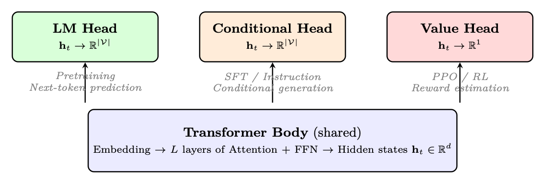
Figure 1.7: The same transformer backbone supports different tasks by swapping the prediction head. All three heads used in this paper share identical architecture below the final projection layer.

P(xt+1|x≤t) = softmax(Whead · ht + b) (1.7)

where Whead ∈R|V|×d (often tied with the embedding matrix: Whead = ET ).

LM Head Properties

• Training objective: Causal language modeling (predict next token for every position)

• Loss: LLM = −1 T PT t=1 log P(xt|x<t)

• Label: Every token is both input (shifted right) and target (shifted left)

• Used during: Pretraining on large corpora (trillions of tokens)

• Key insight: The model learns general language understanding as a byproduct of next-token prediction

1.4.2 Conditional Generation Head (SFT / Instruction Following)

For supervised fine-tuning (SFT), the architecture is identical to the LM head--the same linear projection to vocabulary logits. The difference is purely in what we compute loss on:

|y| X

LSFT = −1

t=1 log P(yt|xprompt, y<t) (1.8)

|y|

Conditional Head - Key Differences from LM Head

• Loss masking: Only compute loss on the response tokens, not the prompt/instruction. The prompt provides context but no gradient signal.

• Conditioning: The model learns to generate responses conditioned on specific instruction formats (system prompts, user queries, tool calls).

• Format tokens: Special tokens (<|user|>, <|assistant|>) guide the model to produce structured outputs.

• Used during: SFT on curated instruction-response pairs; also during RL policy generation (the policy head that produces actions/responses).

Same Head - Different Training Signal

The LM head and SFT head are architecturally identical (same Whead). The only difference is that during SFT, we mask the loss on prompt tokens. This subtle change transforms a general text predictor into a instruction-following assistant. The head learns to "activate" different generation modes based on the conditioning context.

In reinforcement learning (PPO, GRPO), we need to estimate how good a state is--this requires a scalar output, not vocabulary logits. The value head replaces the LM projection with a simple regression layer:

V (st) = wT value · ht + b ∈R (1.9)

where wvalue ∈Rd and b ∈R. Value Head Properties

• Output: Single scalar (expected cumulative reward from this state)

• Loss: MSE between predicted and actual returns: LV = 1 T P t(V (st) −Rt)2

• Architecture: Linear layer Rd →R1 (sometimes with a small MLP: d →256 →1)

• Backbone sharing: Often shares the transformer body with the policy (with a separate value head), or uses a completely separate critic network

• Used during: PPO advantage estimation (GAE), reward model scoring

1.4.4 Head Selection Summary

Table 1.9: Prediction heads used throughout this paper and their training contexts.

Head Output Loss Stage Purpose

LM Head R|V| Cross-entropy (all tokens) Pretraining Learn language from raw text Conditional Head R|V| Cross-entropy (response only) SFT Learn to follow instructions Value Head R1 MSE RL (PPO) Estimate state value for advantage Reward Head R1 Pairwise ranking RM training Score response quality

Head Initialization Matters When adding a value head to a pretrained LM, initialize it near zero (small random weights). If initialized with large values, the initial value estimates will be wildly wrong, causing huge advantages and unstable PPO updates. Common practice: initialize the final linear layer with N(0, 1/ √

d) or simply zeros.

1.4.5 HuggingFace Implementation

from transformers import ( AutoModelForCausalLM , # LM head (pretraining + SFT) AutoModelForSequenceClassification , # Reward head AutoTokenizer , ) from trl import AutoModelForCausalLMWithValueHead # Value head (PPO) import torch

model_name = "meta -llama/Llama -3.1 -8B-Instruct" tokenizer = AutoTokenizer. from_pretrained (model_name)

inputs = tokenizer("The capital of France is", return_tensors ="pt") outputs = lm_model (** inputs) next_token_logits = outputs.logits [:, -1, :] # (batch , vocab_size) probs = torch.softmax(next_token_logits , dim=-1)

# === 2. Conditional Head (SFT) === # Architecturally identical to LM head -- difference is in loss masking # During SFT , we only compute loss on response tokens: messages = [

{"role": "user", "content": "What is 2+2?"}, {"role": "assistant", "content": "4"}, ] formatted = tokenizer. apply_chat_template (messages , return_tensors ="pt") labels = formatted.clone () # Mask prompt tokens (set to -100 so cross -entropy ignores them) prompt_len = len(tokenizer. apply_chat_template (messages [:1])) labels [:, :prompt_len] = -100 loss = lm_model(input_ids=formatted , labels=labels).loss

# === 3. Value Head (PPO Critic) === # Adds a Linear(hidden_size -> 1) on top of the LM backbone value_model = AutoModelForCausalLMWithValueHead . from_pretrained (

model_name , torch_dtype=torch.bfloat16 , device_map="auto", ) # value_model.v_head: Linear(hidden_size -> 1) # Returns both LM logits AND per -token value estimates

inputs = tokenizer("Explain quantum computing", return_tensors ="pt") lm_logits , loss , values = value_model(

**inputs , return_dict=False ) # values shape: (batch , seq_len , 1) -- scalar estimate per token

# === 4. Reward Head (Reward Model) === # Classification head: Linear(hidden_size -> 1) on last token reward_model = AutoModelForSequenceClassification . from_pretrained (

model_name , num_labels =1, # single scalar output torch_dtype=torch.bfloat16 , device_map="auto", ) # Scores entire sequence by pooling the last token 's hidden state inputs = tokenizer("Good response here", return_tensors ="pt") reward_score = reward_model (** inputs).logits # shape: (batch , 1)

Listing 1.3: Loading and using different prediction heads with HuggingFace.

Weight Tying: LM Head = Embedding Matrix Transposed

Most modern LLMs tie the LM head weights with the input embedding matrix: lm_head.weight = model.embed_tokens.weight. This means the LM head is not a separately learned layer--it reuses the embedding table. Benefits: fewer parameters (|V| × d saved), better generalization, and the geometric structure of the embedding space directly determines token probabilities. You can verify this in HuggingFace: model.lm_head.weight is model.model.embed_tokens.weight returns True for most models.

Training a large language model means finding the set of parameters θ (billions of weights) that minimizes the loss function L(θ) -- typically the negative log-likelihood of the next token. This is an optimization problem in extraordinarily high-dimensional space, and the algorithm used to navigate this space determines whether training succeeds, diverges, or stalls.

1.5.1 Gradient Descent: The Foundation

What is a Gradient? The gradient ∇θL is a vector that points in the direction of steepest increase of the loss. Each component ∂L

∂θi tells us how much the loss would change if we slightly increased parameter θi. To decrease the loss, we move in the opposite direction:

θt+1 = θt −η∇θL(θt) (1.10)

where η > 0 is the learning rate -- the step size. This is gradient descent [77].

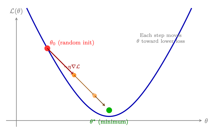
Figure 1.8: Gradient descent: starting from a random initialization θ0, each step moves the parameters in the direction that reduces the loss, with step size controlled by the learning rate η. The process converges toward a (local) minimum.

Why Full Gradient Descent is Impractical. Computing the exact gradient requires evaluating the loss over the entire training dataset (trillions of tokens for LLMs). This is computationally prohibitive -- a single gradient step would require a full pass over all data.

Stochastic Gradient Descent (SGD). The solution: estimate the gradient from a small random subset (mini-batch) of the data [78]:

B X

∇θL(θ) ≈1

i=1 ∇θℓ(θ; xi)

B

where B is the batch size (typically 1K-4M tokens for LLMs). The mini-batch gradient is a noisy but unbiased estimate of the true gradient.

Why Mini-Batch SGD Works

• Computational efficiency: Each step costs O(B) instead of O(Ntotal). With B = 4096 tokens and 15T total tokens, each step is ∼4 billion× cheaper.

• Noise as regularization: The stochastic noise helps escape sharp local minima, finding flatter regions that generalize better.

• GPU utilization: Mini-batches are large enough to saturate GPU parallelism (matrix

• Convergence: Theoretically converges to a local minimum at rate O(1/ √

T) (slower than exact GD's O(1/T), but each step is millions of times cheaper).

From SGD to Adaptive Methods. While SGD with momentum works well for vision models (CNNs), LLM training requires adaptive optimizers -- algorithms that maintain a per-parameter learning rate.

1.5.2 Why Vanilla SGD Fails for LLMs

Stochastic Gradient Descent updates weights as:

θt+1 = θt −η∇θL(θt)

SGD Problems for LLMs

• Different gradient scales per layer: Early layers in a transformer have much smaller gradients than later layers (vanishing gradients). A single learning rate η is too large for some parameters and too small for others.

• Sparse gradients: Embedding layers receive gradients only for tokens in the current batch. Most embedding rows have zero gradient. SGD with momentum wastes momentum on zero-gradient rows.

• Saddle points: High-dimensional loss landscapes have many saddle points. SGD can stall; adaptive methods escape faster.

• Sensitivity to learning rate: SGD requires careful tuning; a 2× change in η can cause divergence.

1.5.3 Adam - Adaptive Moment Estimation

Adam [79] maintains per-parameter estimates of the first moment (mean of gradients) and second moment (uncentered variance of gradients).

Adam Update Equations

Given gradient gt = ∇θL(θt), hyperparameters β1, β2, ϵ, η: Step 1 - Update biased first moment estimate:

mt = β1mt−1 + (1 −β1)gt

Step 2 - Update biased second moment estimate:

vt = β2vt−1 + (1 −β2)g2 t

Step 3 - Bias correction: ˆmt = mt 1 −βt 1 , ˆvt = vt 1 −βt 2 Step 4 - Parameter update:

θt+1 = θt −η · ˆmt √ˆvt + ϵ

Typical values: β1 = 0.9, β2 = 0.95 or 0.999, ϵ = 10−8, η = 10−4 to 10−5.

• mt (momentum): Exponential moving average of gradients. Smooths out noisy gradient estimates. β1 = 0.9 means the current gradient contributes 10% and the history contributes 90%.

• vt (adaptive LR): EMA of squared gradients. Parameters with consistently large gradients get a smaller effective learning rate (η/√vt). Parameters with small gradients get a larger effective LR. This is the key to handling different gradient scales per layer.

• ˆmt, ˆvt (bias correction): At t = 1, m1 = (1 −β1)g1 is much smaller than the true mean. Dividing by (1 −βt 1) corrects this initialization bias. Without it, early steps are too small.

• ϵ (numerical stability): Prevents division by zero. Also acts as a floor on the effective learning rate.

1.5.4 AdamW - Decoupled Weight Decay

AdamW [80] fixes a subtle but important issue with how weight decay interacts with adaptive optimizers.

Why L2 Regularization ̸= Weight Decay in Adam

With L2 regularization, the loss becomes L + λ

2∥θ∥2, so the gradient is gt + λθt. In Adam, this regularization gradient is scaled by the adaptive factor 1/√ˆvt:

θt+1 = θt −η · ˆmt + λθt √ˆvt + ϵ

Parameters with large vt (large gradient variance) get less regularization. This is not what we want - weight decay should be uniform.

AdamW - Decoupled Weight Decay

AdamW (Loshchilov & Hutter, 2017) applies weight decay directly to the parameters, outside the adaptive scaling:

θt+1 = θt −η · ˆmt √ˆvt + ϵ −ηλθt

The weight decay term ηλθt is not divided by √ˆvt. This gives uniform regularization across all parameters regardless of their gradient history. Typical value: λ = 0.1 for LLM training.

Always Use AdamW - Never Plain Adam - for LLMs

The difference between Adam and AdamW is subtle but matters. With Adam + L2, the effective weight decay is stronger for parameters with small gradient variance (e.g., biases, LayerNorm parameters) and weaker for parameters with large gradient variance (e.g., attention weights). AdamW gives the intended uniform regularization. Most frameworks default to AdamW; doublecheck your optimizer class.

Typical Learning Rates by Training Phase

Phase Typical LR Notes

Pretraining (from scratch) 1e-4 to 3e-4 Large model, large batch Continued pretraining 1e-5 to 1e-4 Smaller LR to preserve knowledge SFT (supervised fine-tune) 1e-5 to 2e-5 Standard range LoRA fine-tuning 1e-4 to 3e-4 Higher LR for adapter weights

For RL learning rates (PPO, DPO, GRPO) see §11.15.

1.5.6 Learning Rate Warmup

Why Warmup is Necessary

At the start of training, vt (the second moment estimate) is initialized to zero. After bias correction: ˆvt = vt/(1−βt 2). At t = 1 with β2 = 0.999: ˆv1 = v1/(1−0.999) = 1000v1. This means the effective learning rate is η/√1000v1 - much smaller than intended. However, if the first gradient is unusually large (common at initialization), the second moment estimate can be dominated by this outlier, causing erratic early steps. Warmup mitigates this by starting with a very small LR and gradually increasing it, giving vt time to accumulate a reliable estimate.

• Linear warmup: ηt = ηmax × t/Twarmup

• Typical warmup duration: 1-5% of total steps for pretraining; 3-10% for fine-tuning (shorter runs need proportionally more warmup)

• For SFT: 50-200 warmup steps is typical

1.5.7 Learning Rate Schedules

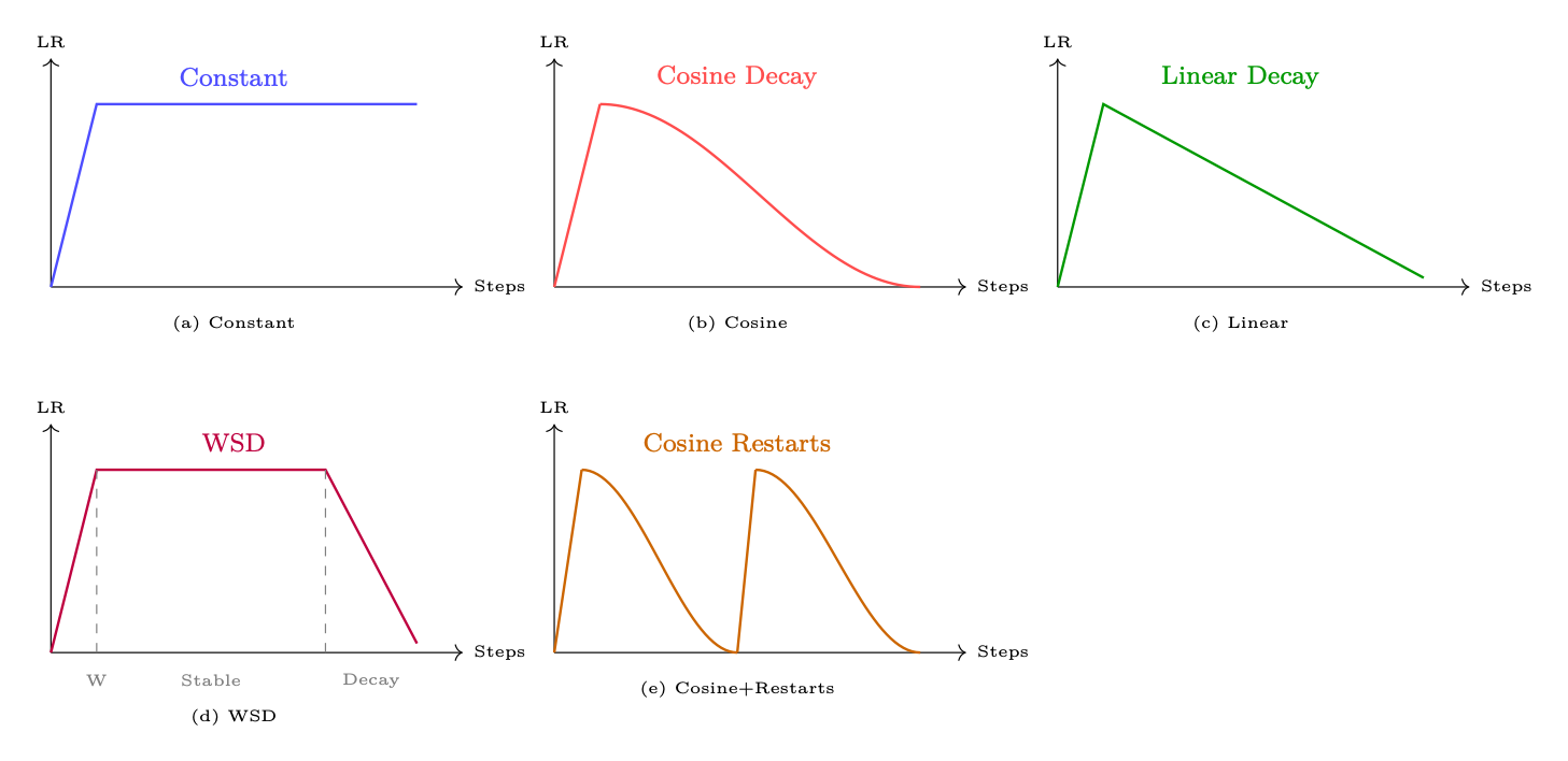
Figure 1.9: Common learning rate schedules. All include a linear warmup phase. WSD (Warmup-StableDecay) is the emerging standard for pretraining.

t −Twarmup T −Twarmup π

!!

ηt = ηmin + 1

2(ηmax −ηmin)

1 + cos

Standard for pretraining and SFT. Smooth decay avoids abrupt LR changes. ηmin is typically ηmax/10.

(c) Linear Decay. Simpler than cosine, similar empirical results. Preferred when you want predictable LR at any step.

(d) WSD - Warmup-Stable-Decay. The new standard for large-scale pretraining [25, 81]. Three phases:

1. Warmup: Linear ramp to ηmax (1-5% of steps)

2. Stable: Constant ηmax for the majority of training

3. Decay: Fast cosine or linear decay to ηmin (last 10-20% of steps)

Key advantage: the stable phase allows checkpointing at any point and continuing training. The decay phase can be applied at the end of any run.

(e) Cosine with Restarts (SGDR). Periodic restarts reset the LR to ηmax. Can help escape local minima. Less common for LLMs; more useful for smaller models.

1.5.8 Gradient Clipping

Gradient Clipping

Gradient clipping rescales the gradient if its global norm exceeds a threshold:

gt ←gt · min � 1, τ ∥gt∥2

�

where τ is max_grad_norm (typically 1.0).

Gradient Clipping vs. LR Reduction

Gradient clipping and reducing the learning rate both limit the size of parameter updates. The difference: clipping preserves the direction of the gradient (just scales the magnitude), while a smaller LR scales all updates uniformly. Clipping is better for handling occasional large gradients without slowing down normal training steps.

Putting It Together: HuggingFace Optimizer Configuration

The following snippet shows how the concepts from this section--AdamW with decoupled weight decay (§1.6.6), cosine learning-rate scheduling with linear warmup (§1.6.7), and gradient clipping (§1.6.8)--come together in practice using the HuggingFace transformers library.

from transformers import TrainingArguments , Trainer from transformers import get_cosine_schedule_with_warmup import torch

# --- Option 1: Using TrainingArguments (recommended) --- training_args = TrainingArguments (

output_dir="./ checkpoints",

# Learning rate schedule (S1 .6.7) lr_scheduler_type ="cosine", # cosine decay to 0 warmup_ratio =0.1, # 10% of steps = linear warmup

# Gradient clipping (S1 .6.8) max_grad_norm =1.0, # clip by global L2 norm

# Mixed precision (S1 .6.9) bf16=True , # use BFloat16 on Ampere+ GPUs

# Training duration num_train_epochs =3, per_device_train_batch_size =8, gradient_accumulation_steps =4, # effective batch = 8*4 = 32 )

trainer = Trainer(

model=model , args=training_args , train_dataset=dataset , ) trainer.train ()

# --- Option 2: Manual control (for custom training loops) --- from torch.optim import AdamW

# Separate weight -decay groups (don't regularize biases/norms) no_decay = ["bias", "LayerNorm.weight", "layernorm.weight"] param_groups = [

{

"params": [p for n, p in model. named_parameters ()

if not any(nd in n for nd in no_decay)], "weight_decay": 0.01, }, {

"params": [p for n, p in model. named_parameters ()

if any(nd in n for nd in no_decay)], "weight_decay": 0.0, }, ]

optimizer = AdamW(param_groups , lr=2e-5, betas =(0.9 , 0.999))

# Cosine schedule with linear warmup total_steps = len( train_dataloader ) * num_epochs warmup_steps = int (0.1 * total_steps) scheduler = get_cosine_schedule_with_warmup (

optimizer , num_warmup_steps =warmup_steps , num_training_steps =total_steps , )

# Training loop with gradient clipping for batch in train_dataloader :

outputs = model (** batch) loss = outputs.loss loss.backward ()

# Clip gradients before optimizer step torch.nn.utils. clip_grad_norm_ (model.parameters (), max_norm =1.0)

optimizer.step () scheduler.step () optimizer.zero_grad ()

Listing 1.4: Complete optimizer configuration combining AdamW - cosine schedule - and gradient clipping.

Practical Tips

• Weight decay exclusion: bias terms and layer-norm weights should not be regularized-- they have few parameters and regularizing them hurts performance [80].

• Warmup ratio: 5-10% of total steps is standard; too little warmup with a high LR can destabilize early training.

• Gradient accumulation: simulates larger batches on limited GPU memory; clipping applies to the accumulated gradient.

• BF16 vs. FP16: prefer bf16=True on Ampere+ GPUs (wider dynamic range avoids loss scaling); fall back to fp16=True on older hardware.

1.5.9 Mixed Precision Training

BF16 vs. FP16

Format Exponent bits Mantissa bits Dynamic range

FP32 8 23 ∼10−38 to 1038

BF16 8 7 Same as FP32 (same exponent) FP16 5 10 ∼6 × 10−5 to 65504

BF16 Over FP16: Why Range Beats Precision in LLM Training

BF16 has the same exponent range as FP32, so it can represent the same range of values (just with less precision in the mantissa). FP16 has a much smaller dynamic range - gradients or activations that exceed 65504 cause overflow (NaN/Inf). This is why FP16 training requires loss scaling (multiplying the loss by a large constant to keep gradients in FP16 range), while BF16 training typically does not. A100 and H100 support BF16 natively; use BF16 unless you have a specific reason for FP16.

Loss Scaling (FP16 only).

1. Multiply loss by scale factor S (e.g., S = 215)

2. Compute gradients in FP16 (scaled by S)

3. Before optimizer step, divide gradients by S

4. Check for overflow (NaN/Inf); if found, skip step and reduce S

5. If no overflow for N consecutive steps, increase S

FP32 Master Weights. In mixed precision training, weights are stored in FP32 (master copy) and cast to BF16/FP16 for the forward/backward pass. The optimizer step is done in FP32. This is important because:

• Memory cost: 2× weight storage (FP32 + BF16 copy)

When FP32 Master Weights Are Critical

FP32 master weights are most important for:

• Long training runs (many small gradient steps accumulate)

• Small learning rates (updates are tiny relative to weight magnitude)

For short SFT runs with large LR, BF16-only training (no FP32 master weights) often works fine and saves memory. For RL training, FP32 master weights are essential--see §11.15.

Mixed Precision in Practice: HuggingFace

# === HuggingFace TrainingArguments (simplest approach) === from transformers import TrainingArguments

# BF16 on Ampere+ GPUs (A100 , H100 , RTX 30xx/40xx) args_bf16 = TrainingArguments (

output_dir="./out", bf16=True , # BF16 forward/backward; FP32 master weights bf16_full_eval =True , # also use BF16 during evaluation # No loss scaling needed -- BF16 has FP32 -equivalent range )

# FP16 on older GPUs (V100 , T4 , RTX 20xx) args_fp16 = TrainingArguments (

output_dir="./out", fp16=True , # FP16 forward/backward fp16_full_eval =False , # keep eval in FP32 for accuracy # Loss scaling is automatic via PyTorch GradScaler )

# === Manual PyTorch AMP (for custom training loops) === import torch

# Setup (PyTorch 2.x API) use_fp16 = not torch.cuda. is_bf16_supported () scaler = torch.amp.GradScaler("cuda", enabled=use_fp16) # only needed for FP16 optimizer = torch.optim.AdamW(model.parameters (), lr=2e-5) dtype = torch.float16 if use_fp16 else torch.bfloat16

for batch in train_dataloader :

optimizer.zero_grad ()

# Autocast: run forward pass in reduced precision with torch.autocast("cuda", dtype=dtype): outputs = model (** batch) loss = outputs.loss

if use_fp16:

# FP16 path: scale loss to prevent gradient underflow scaler.scale(loss).backward () scaler.unscale_(optimizer) # unscale before clipping torch.nn.utils. clip_grad_norm_ (model.parameters (), 1.0) scaler.step(optimizer) # skips step on overflow scaler.update () # adjust scale factor else:

scheduler.step ()

Listing 1.5: Mixed precision training with HuggingFace and manual PyTorch AMP.

Key Differences: BF16 vs. FP16 in Code

• BF16: just wrap with autocast(dtype=torch.bfloat16)--no scaler needed. Simpler code and more numerically stable.

• FP16: requires GradScaler to prevent gradient underflow. The scaler dynamically adjusts a multiplier; if overflow is detected (NaN), the optimizer step is skipped and the scale is reduced.

• Gradient clipping + FP16: you must call scaler.unscale_(optimizer) before clip_grad_norm_, otherwise you're clipping scaled gradients (wrong threshold).

• Memory savings: % reduction in activation memory (activations stored in 16-bit); weight memory depends on whether you keep FP32 master copies.

1.5.10 Practical Optimizer Settings by Training Phase

Optimizer Hyperparameter Reference Table

Phase Optimizer LR WD Warmup Schedule

Pretraining AdamW 3e-4 0.1 2000 steps WSD or Cosine SFT AdamW 2e-5 0.01 100 steps Cosine LoRA SFT AdamW 2e-4 0.01 100 steps Cosine

All use: β1=0.9, β2=0.95, ϵ=10−8, max_grad_norm=1.0, BF16. For RL settings see §11.15.

Diagnosing Training Instability

# Monitor these metrics to diagnose optimizer issues: # 1. Gradient norm -- should be < max_grad_norm most of the time # 2. Loss scale (FP16) -- should be stable , not constantly decreasing # 3. Parameter update norm -- should be << parameter norm

import torch

def log_optimizer_stats (model , optimizer , step): # Gradient norm (before clipping) total_norm = 0.0 for p in model.parameters ():

if p.grad is not None:

total_norm += p.grad.data.norm (2).item () ** 2 total_norm = total_norm ** 0.5

# Adam second moment stats (proxy for adaptive LR) v_norms = [] for group in optimizer.param_groups :

for p in group['params ']:

state = optimizer.state[p] if 'exp_avg_sq ' in state:

v_norms.append(state['exp_avg_sq ']. mean ().item ())

print(f"Step {step }: grad_norm ={ total_norm :.3f}, "

f"mean_v ={sum(v_norms)/len(v_norms):.6f}")

# Red flags:

The Learning Rate is the Most Important Hyperparameter

In practice, getting the learning rate right matters more than any other hyperparameter. A rule of thumb for LLM fine-tuning:

• Start with the values in the table above

• If loss diverges (increases after initial decrease): LR is too high

• If loss decreases very slowly and plateaus early: LR is too low

• If loss is unstable (oscillates): LR is too high or warmup is too short

The second most important hyperparameter is batch size (affects gradient noise and effective LR via the linear scaling rule). Everything else is secondary.

1.6 Flash Attention - Algorithm and Hardware Awareness

Flash Attention [7, 82] is one of the most impactful algorithmic innovations in deep learning since the transformer itself. It does not change the mathematical result of attention - it computes exactly the same output - but it restructures the memory access pattern so that the GPU's limited fast SRAM does all the heavy lifting, cutting HBM footprint from O(n2) to O(n) and delivering 2-4× end-to-end wall-clock gains on typical workloads.

1.6.1 The Standard Attention Memory Problem

Standard scaled dot-product attention is:

QKT

!

√dk

Attention(Q, K, V ) = softmax

V

Standard Attention Memory Complexity

For sequence length n and head dimension d:

• Q, K, V ∈Rn×d: O(nd) memory

• S = QKT ∈Rn×n: O(n2) memory - the bottleneck

• P = softmax(S) ∈Rn×n: another O(n2)

• O = PV ∈Rn×d: O(nd)

At n = 8192, d = 128, BF16: the attention matrix alone is 81922 × 2 ≈134 MB per head. With 32 heads, that is 4.3 GB just for one layer's attention scores.

Why O(n2) is Catastrophic

The attention matrix must be written to HBM (it does not fit in SRAM for long sequences), then read back for the softmax, then read again for the PV product. Each of these HBM round-trips is slow. For n = 32768 (32K context), the attention matrix is 327682 × 2 ≈2 GB per head completely infeasible to store.

The core insight is: we never need the full n × n matrix in memory at once. We can compute the output O block-by-block if we use the online softmax trick.

Online Softmax. Recall that softmax requires a global maximum for numerical stability:

softmax(xi) = exi−m P j exj−m , m = max j xj

The trick: we can update the running maximum and normalization factor as we process new blocks, without ever materializing the full row.

Online Softmax Update Rule

Given a running state (mold, ℓold, Oold) and a new block of scores snew:

1. mnew = max(mold, max(snew))

2. ℓnew = emold−mnew · ℓold + P _jes_new,j−m_new

� em_old−m_new · ℓ_old · O_old + es_new−m_new · V _new �

3. Onew = 1 ℓnew

This is mathematically equivalent to computing softmax over all blocks at once.

1.6.3 The Flash Attention Algorithm

Flash Attention Forward Pass - Block Tiling

Setup: SRAM size M. Block sizes Br = ⌈M/(4d)⌉, Bc = min(⌈M/(4d)⌉, d).

1. Divide Q into Tr = ⌈n/Br⌉blocks Q1, . . . , QTr

2. Divide K, V into Tc = ⌈n/Bc⌉blocks K1, . . . , KTc

3. Initialize output O ∈Rn×d, running max m ∈Rn, running sum ℓ∈Rn (all in HBM)

4. Outer loop over j = 1, . . . , Tc:

(a) Load Kj, Vj from HBM to SRAM

(b) Inner loop over i = 1, . . . , Tr:

i. Load Qi, Oi, mi, ℓi from HBM to SRAM ii. Compute Sij = QiKT j / √

d (stays in SRAM) iii. Apply online softmax update to get new mi, ℓi, Oi iv. Write Oi, mi, ℓi back to HBM

5. Return O

Key: Sij (the attention tile) is computed and discarded in SRAM. It is never written to HBM.

Flash Attention Complexity

Standard Attention Flash Attention

Memory (HBM) O(n2) O(n) HBM reads/writes O(n2d) O(n2d/M) FLOPs O(n2d) O(n2d) (same) Speedup 1× 2-4×

1.6.4 Flash Attention 2 - Better Parallelism

Flash Attention 2 [82] made three key improvements:

1. Reduced non-matmul FLOPs: The original FA had unnecessary rescaling operations in the inner loop. FA2 restructures the loop to minimize these. On A100, Tensor Core matrix multiplications outpace scalar operations by roughly 16×, so even a small fraction of non-matmul work in the inner loop becomes the latency bottleneck.

2. Better parallelism across sequence dimension: FA1 parallelized over batch and heads only. FA2 also parallelizes over the query sequence dimension, enabling better GPU utilization for long sequences with small batch sizes.

3. Causal masking optimization: For autoregressive (causal) attention, roughly half the blocks are fully masked. FA2 skips these blocks entirely, giving ∼2× speedup for causal attention vs. bidirectional.

1.6.5 Flash Attention 3 - Hopper Architecture

Flash Attention 3 [83] is designed specifically for H100 and exploits three Hopper-specific features:

• TMA (Tensor Memory Accelerator): H100 has a dedicated hardware unit for asynchronous bulk data movement between HBM and SRAM. FA3 uses TMA to overlap data loading with computation, hiding memory latency.

• Warp-specialization: FA3 assigns different warps to different roles (producer warps load data via TMA; consumer warps compute MMA). This is a software pipelining technique that keeps both the memory system and Tensor Cores busy simultaneously.

• FP8 support: H100 supports FP8 (E4M3/E5M2) Tensor Core operations at 2× the throughput of BF16. FA3 supports FP8 attention with per-block quantization to maintain accuracy.

FA3 achieves up to 75% of H100 theoretical peak for FP16 attention, compared to ∼35% for FA2.

1.6.6 Flash Attention 4 - Blackwell Architecture

Flash Attention 4 [84] targets NVIDIA's Blackwell GPUs (B200/GB200), which double Tensor Core throughput to 2.25 PFLOP/s (BF16) while non-matmul units (exponential, shared memory bandwidth) scale at a slower rate. This asymmetric hardware scaling means that the bottleneck shifts: on Blackwell, attention is limited not by matmul but by the softmax exponentials and shared memory traffic surrounding them. FA4 addresses this with four key techniques:

• Fully asynchronous MMA pipelines: Blackwell's MMA instructions are fully asynchronous (unlike Hopper's wgmma which still blocked on completion). FA4 redesigns the pipeline to overlap MMA, TMA loads, and softmax rescaling across larger tile sizes, keeping all hardware units saturated.

• Tensor Memory + 2-CTA MMA mode (backward pass): The backward pass uses Blackwell's Tensor Memory (a per-SM scratchpad larger than shared memory) and a 2-CTA cooperative mode that fuses dQ accumulation across two thread-block clusters, halving shared memory round-trips.

FA4 Implementation: CuTe-DSL

FA4 is the first FlashAttention version written in CuTe-DSL, a Python-embedded domain-specific language for GPU kernels (part of CUTLASS 4.x). CuTe-DSL compiles 20-30× faster than C++ CUTLASS templates while retaining full control over register allocation and pipeline scheduling. This dramatically lowers the iteration time for kernel development.

Results. On B200 with BF16 head-dim 128 (causal, seq-len 8K):

• 1613 TFLOP/s - 71% of Blackwell peak utilization

• 1.3× faster than cuDNN 9.13 (NVIDIA's proprietary fused kernel)

• 2.7× faster than Triton on the same hardware

Hardware-Software Co-evolution The FlashAttention series illustrates a key principle: each GPU generation shifts the bottleneck, demanding new algorithmic ideas rather than just re-compilation. A80 →memory bandwidth limited (FA1/FA2: tiling + recomputation). H100 →data movement limited (FA3: TMA + warpspecialization). B200 →non-matmul compute limited (FA4: software-emulated exp + conditional rescaling). Understanding where the hardware bottleneck lies is the prerequisite for writing efficient kernels.

1.7 Pretraining: Best Practices

Pretraining is the most expensive phase of LLM development--consuming millions of GPU-hours and requiring careful orchestration of data, compute, and hyperparameters. This section distills key lessons from Llama-3 [25], Chinchilla [85], and GPT-4 [23].

1.7.1 Training Objective

All modern decoder-only LLMs use causal language modeling (CLM):

T X

LCLM = −1

t=1 log Pθ(xt | x<t)

T

This simple objective--with enough data and scale--produces emergent capabilities (in-context learning, reasoning, instruction following) without explicit supervision [21].

1.7.2 Data Pipeline

Pretraining Data Recipe

• Scale: 1-15 trillion tokens for frontier models (Llama-3: 15T tokens)

• Sources: Web crawl (80%), code (10%), books/papers (5%), curated (5%)

• Deduplication: MinHash + exact substring dedup reduces memorization [86]

• Data mixing: Temperature-weighted sampling across domains; upweight code and math for reasoning

1.7.3 Scaling Laws

Hoffmann et al. [85] showed that compute-optimal training requires balancing model size N and data size D: Nopt ∝C0.50, Dopt ∝C0.50. A 70B model is compute-optimal at ∼1.4T tokens. In practice, models are over-trained (more tokens than Chinchilla-optimal) because inference cost scales with model size, not training tokens--smaller over-trained models are cheaper to deploy.

1.7.4 Key Hyperparameters

Table 1.10: Pretraining hyperparameters from published models.

Setting Llama-3 405B Llama-3 8B Qwen-2.5 72B Mistral 7B

Tokens 15T 15T 18T 8T Batch size (tokens) 16M 4M 4M 4M Peak LR 8e-5 3e-4 3e-4 3e-4 Schedule WSD WSD Cosine Cosine Weight decay 0.1 0.1 0.1 0.1 Context length 8192 8192 4096→32K 8192

1.7.5 Common Failure Modes

Pretraining Pitfalls

• Loss spikes: Sudden loss increases from bad data batches or numerical instability. Llama-3 reports rolling back to checkpoints and skipping offending batches.

• Memorization: Model regurgitates training data verbatim. Fix: deduplicate aggressively; monitor extraction attacks.

• Context length: Training on short sequences then deploying at long context fails. Use continued pretraining on long documents + RoPE scaling.

1.8 Supervised Fine-Tuning (SFT)

SFT transforms a pretrained language model into an instruction-following assistant by training on curated prompt-response pairs. This is the bridge between raw language modeling and RLHF.

1.8.1 SFT Objective

The loss is identical to CLM, but computed only on response tokens:

|y| X

LSFT = −1

t=1 log Pθ(yt | xprompt, y<t)

|y|

Prompt tokens provide context but receive no gradient (labels set to −100).

1.8.2 Data Quality: The LIMA Principle

• Correctness: Every response must be factually accurate and well-formatted

• Length balance: Mix short (1-sentence) and long (multi-paragraph) responses

• Decontamination: Remove overlap with evaluation benchmarks

1.8.3 Training Configuration

from trl import SFTTrainer , SFTConfig

sft_config = SFTConfig(

output_dir="./ sft_output", max_seq_length =4096 , packing=True , # Pack short examples into full sequences learning_rate =2e-5, lr_scheduler_type ="cosine", warmup_ratio =0.1, weight_decay =0.01 , max_grad_norm =1.0, num_train_epochs =3, per_device_train_batch_size =4, gradient_accumulation_steps =8, bf16=True , gradient_checkpointing =True , ) trainer = SFTTrainer(model=model , args=sft_config ,

train_dataset =dataset , processing_class =tokenizer) trainer.train ()

1.8.4 Efficient Training Solutions

Standard HuggingFace training leaves significant performance on the table. Several libraries provide drop-in efficiency gains for SFT workloads:

Liger Kernel [88]. An open-source set of Triton-fused kernels from LinkedIn that replace standard PyTorch operators during training. Key fusions include:

• Fused Cross-Entropy: Merges the final linear projection, softmax, and loss computation into a single kernel--avoids materializing the full (batch × seq × vocab) logit tensor.

• Fused RMSNorm / SwiGLU / RoPE: Eliminates intermediate memory allocations for common LLM building blocks.

• Chunked operations: Processes large tensors in tiles to keep peak memory bounded.

Result: 20% higher throughput and up to 60% memory reduction with a one-line integration (apply_liger_kernel_to_llama()). Compatible with FSDP, DeepSpeed, and LoRA.

Unsloth [89]. A specialized fine-tuning library that combines custom CUDA/Triton kernels with aggressive memory optimization:

• Manual backpropagation through LoRA layers (avoids autograd overhead).

• 4-bit QLoRA with fused dequantization--trains 70B models on a single 48 GB GPU.

• Intelligent RoPE and attention kernel fusion specific to each architecture (Llama, Mistral, Qwen, Gemma).

• Pure PyTorch--no trainer class; recipes are readable single-file scripts.

• Native integration with torch.compile, FSDP2, and activation checkpointing.

• First-class support for QLoRA, full fine-tuning, and knowledge distillation.

• Built-in quantization-aware training (QAT) for post-training compression.

Result: Comparable speed to custom solutions but with full debuggability and no framework lock-in.

Choosing an Efficiency Stack

• Quick LoRA/QLoRA on ≤1 GPU: Unsloth (fastest time-to-train, minimal setup)

• Multi-GPU full fine-tune: TRL/DeepSpeed + Liger Kernel (best throughput at scale)

• Research / custom training loops: torchtune (transparent, hackable, native PyTorch)

These are complementary: Liger kernels can be used inside both TRL and torchtune workflows.

1.8.5 Best Practices

Table 1.11: SFT training guidelines.

Practice Details

Packing Concatenate multiple short examples into one sequence (separated by EOS). Avoids padding waste. NEFTune [91] Add uniform noise to embeddings (α = 5). Improves MT-Bench by 5-15% at zero cost. Chat template Always use the model's native template. Mismatched templates degrade quality. Epochs 2-3 for large datasets; up to 5 for small (<10K) curated sets. Overtraining causes format memorization.

SFT Is Not Enough

SFT teaches format and basic instruction following, but cannot reliably teach: preference (which response is better--needs RLHF/DPO), refusal (when not to answer--needs safety training), calibration (saying "I don't know"--needs RL with truthfulness rewards), or complex reasoning (multi-step chains--needs RL with verifiable rewards). The full pipeline is: Pretrain →SFT → RLHF/DPO.

1.9 LoRA and Parameter-Efficient Fine-Tuning

Full fine-tuning of a 70B model requires storing 70B trainable parameters plus their optimizer states (560+ GB of memory). LoRA [92] (Low-Rank Adaptation) provides a way to fine-tune with <1% of the parameters while achieving comparable quality.

1.9.1 The LoRA Insight

LoRA Core Idea

Instead of updating a full weight matrix W ∈Rd×d, learn a low-rank perturbation:

W ′ = W + α

• Only B and A are trained: 2 × d × r parameters instead of d2

• At rank r = 16, d = 4096: LoRA adds 2 × 4096 × 16 = 131K params per layer vs. 16.8M for full matrix

• α/r scaling controls the magnitude of the update

Why Low-Rank Works

Aghajanyan et al. [93] showed that fine-tuning operates in a very low-dimensional subspace -- the "intrinsic dimensionality" of the fine-tuning task is much smaller than the model's parameter count. A 175B model's fine-tuning task may have intrinsic dimensionality <10,000. LoRA exploits this directly: rank r constrains the update to an r-dimensional subspace per weight matrix.

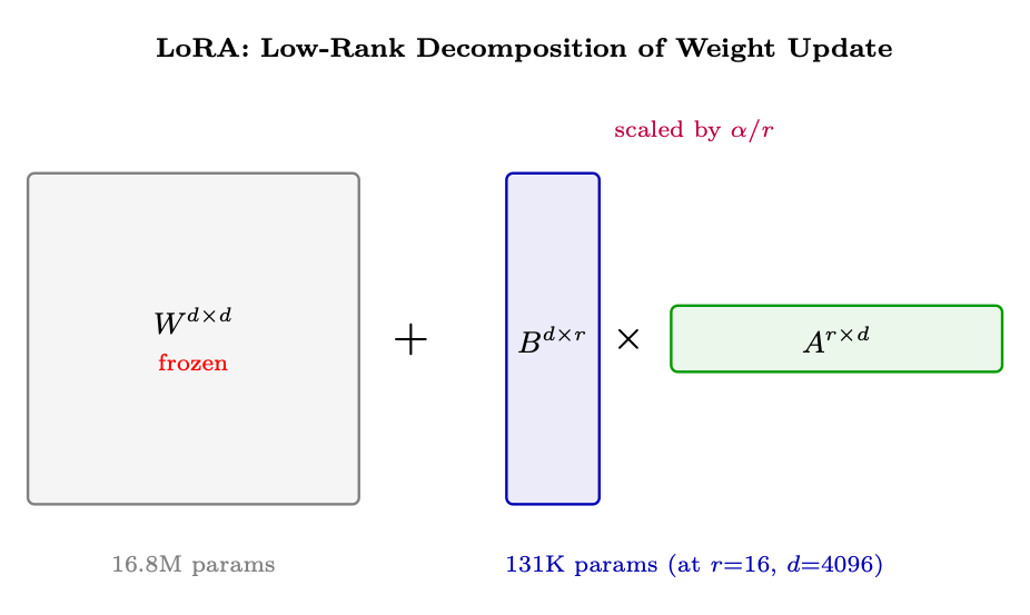
Figure 1.10: LoRA decomposes the weight update ∆W into two small matrices B × A. The original weight W remains frozen; only B and A receive gradients. At inference, the product BA can be merged into W with zero overhead.

Why the α/r Scaling Matters

Without scaling, doubling the rank r would roughly double the magnitude of ∆W = BA (more columns in B contribute to the sum). This means changing rank would also change how much the model is perturbed--you'd need to re-tune the learning rate every time you adjust r. The α/r factor normalizes the update magnitude so that it stays approximately constant regardless of rank: W ′ = W + α

r · BA

• Fix α, sweep r: The effective update magnitude stays ∼α regardless of rank. You can try r ∈{8, 16, 32, 64} without re-tuning LR.

• Common practice: Set α = r (so α/r = 1) or α = 2r (so α/r = 2). This is a convenient default where the scaling factor is a small integer.

• Why not just tune LR? You could, but α/r provides a rank-independent knob. Teams can share LR recipes across experiments with different ranks.

• rsLoRA insight [94]: At high ranks (r ≥64), empirical evidence shows α/√r is more stable than α/r, because the variance of BA scales with √r, not r.

Choosing LoRA hyperparameters correctly is critical -- the wrong rank or alpha can either under-fit (too constrained) or waste memory (too expressive).

Table 1.12: LoRA hyperparameter guide.

Hyperparameter Typical Values Guidance

r (rank) 8, 16, 32, 64 Higher = more capacity but more memory. Start with 16. lora_alpha 16, 32 (often = r or 2r) Controls update magnitude via α/r scaling. target_modules q_proj, k_proj, v_proj, o_proj All attention projections. Add gate_proj, up_proj, down_proj for full coverage. lora_dropout 0.0-0.1 Regularization. Usually 0.05 for small datasets. bias "none" Training biases adds minimal params but rarely helps. Learning rate 1e-4 to 3e-4 Higher than full fine-tuning (only adapters update).

Rank Selection Rules of Thumb

• r=8: Simple tasks (single-domain chat, classification). Very memory-efficient.

• r=16: General-purpose fine-tuning. Good default.

• r=32-64: Complex tasks (math, code, multi-turn reasoning). Approaches full fine-tune quality.

• r=128+: Diminishing returns; consider full fine-tuning or QLoRA with higher rank.

• Key indicator: If training loss plateaus well above full fine-tune loss, increase rank.

1.9.3 LoRA Variants

Table 1.13: LoRA variants and their innovations.

Method Key Innovation When to Use

QLoRA [95] 4-bit quantized base + LoRA in BF16. NF4 data type + double quantization.

Fine-tune 70B on single 48GB GPU.

DoRA [96] Decomposes W into magnitude and direction; LoRA updates direction only.

Better generalization for reasoning.

LoRA+ [97] Different LRs for A/B (ηB = ληA, λ ≈16). Free 2% gain; no extra cost.

AdaLoRA [98] Dynamic rank budget across layers (SVD-based importance).

Very tight compute budget.

rsLoRA [94] Scales by α/√r instead of α/r. Stable at high ranks. When using r ≥64.

VeRA [99] Shared frozen random A, B; trains diagonal scaling only. Extreme param efficiency.

LoRA-FA Freezes A after init; only trains B. Halves LoRA memory. Memory-constrained scenarios.

DoRA - Weight-Decomposed Low-Rank Adaptation. DoRA [96] observes that full finetuning tends to change the direction of weight vectors more than their magnitude. Standard LoRA conflates both. DoRA decomposes each weight column into magnitude m = ∥W∥col and direction ˆV = W/∥W∥col, then applies LoRA only to the direction:

W ′ = m ⊙ˆV ′, ˆV ′ = W + BA ∥W + BA∥col

Magnitude m is a separate learnable vector (one scalar per column). This consistently outperforms LoRA by 1-3% on reasoning and instruction-following benchmarks with no additional inference cost (merged at deployment).

# LoRA+ in PEFT: set different LRs per matrix optimizer_grouped_parameters = [

{"params": [p for n, p in model. named_parameters () if "lora_B" in n],

"lr": 2e-4 * 16}, # B matrix: higher LR {"params": [p for n, p in model. named_parameters () if "lora_A" in n],

"lr": 2e-4}, # A matrix: base LR ]

VeRA - Vector-based Random Matrix Adaptation. VeRA [99] takes parameter efficiency to the extreme: instead of learning A and B, it freezes them as shared random matrices across all layers and only trains two diagonal scaling vectors db ∈Rr and da ∈Rd:

∆W = B · diag(db) · A · diag(da)

This reduces trainable parameters by ∼10× vs. LoRA (only r + d params per layer) while achieving 90-95% of LoRA quality. Best for scenarios where you need hundreds of task-specific adapters with minimal storage.

QLoRA Memory Savings

70B model full fine-tune: 140 GB (weights) + 280 GB (optimizer) + 140 GB (gradients) = 560 GB (7× A100-80GB). 70B QLoRA (r=16, all linear layers):

• Base model in NF4: 70B × 0.5 = 35 GB

• LoRA adapters in BF16: ∼160 MB

• Optimizer states (only for adapters): ∼320 MB

• Activations (gradient checkpointing): ∼8 GB

• Total: ∼44 GB -- fits in a single 48GB GPU!

# QLoRA configuration with PEFT from peft import LoraConfig , get_peft_model , prepare_model_for_kbit_training from transformers import BitsAndBytesConfig import torch

# 4-bit quantization config bnb_config = BitsAndBytesConfig (

load_in_4bit=True , bnb_4bit_quant_type ="nf4", # NormalFloat4 - optimal for weights bnb_4bit_compute_dtype =torch.bfloat16 , # Compute in BF16 bnb_4bit_use_double_quant =True , # Quantize the quantization constants )

# LoRA config lora_config = LoraConfig(

r=16, lora_alpha =32, # alpha/r = 2x scaling target_modules =["q_proj", "k_proj", "v_proj", "o_proj",

"gate_proj", "up_proj", "down_proj"], lora_dropout =0.05 , bias="none", task_type="CAUSAL_LM", )

1.9.4 Other PEFT Approaches

LoRA dominates modern practice, but it is not the only parameter-efficient method. For completeness, the main alternatives: Table 1.14: PEFT method families. LoRA is the de facto standard for LLM fine-tuning; the others are included for historical context and niche use cases.

Method Mechanism Pros / Cons Status

LoRA [92] (and variants) Low-rank matrices added to existing weights

Mergeable at inference (zero overhead); well-supported; works for all architectures

Standard

Adapters [100] Small bottleneck MLPs inserted between layers

Modular; stackable; adds inference latency (extra sequential layers)

Rarely used

Prefix Tuning [101] Learnable "virtual tokens" prepended to keys/values at each layer

No weight modification; effective for generation tasks; consumes context length

Niche

Prompt Tuning [102] Learnable soft prompt embeddings prepended to input

Extremely few params (<0.01%); weaker than LoRA for complex tasks

Niche

IA3 [103] Learned vectors that rescale keys, values, and FFN activations

Even fewer params than LoRA; mergeable; limited capacity

Deprecated

BitFit [104] Train only bias terms Near-zero params; surprisingly effective for simple tasks; limited expressiveness

Historical

Why LoRA Won

LoRA became the standard because it uniquely combines: (1) zero inference overhead -- adapters merge into base weights, unlike Adapters or Prefix Tuning which add latency or consume context; (2) composability -- multiple LoRA adapters can be swapped at serving time for multi-tenant deployments; (3) ecosystem support -- HuggingFace PEFT, TRL, vLLM, and all major frameworks have first-class LoRA support; (4) proven at scale -- used in production by Meta, Google, and most open-source fine-tunes on HuggingFace. Unless you have a specific constraint that LoRA cannot satisfy, it should be your default choice.

Mixture of Experts models [105, 106] scale model capacity without proportionally scaling compute cost by activating only a subset of parameters for each token.

1.10.1 Architecture

MoE Layer

In a MoE transformer, the FFN layer in each block is replaced by N parallel "expert" FFNs plus a router that selects which experts to use:

N X

MoE(x) =

i=1 gi(x) · Ei(x), g(x) = TopK(softmax(Wrx))

• Ei are expert networks (standard FFN layers)

• gi(x) are gating weights from the router (only top-K are non-zero)

• Typically K = 2 out of N = 8-64 experts are active per token

• Total params scale with N; active params scale with K/N of FFN size

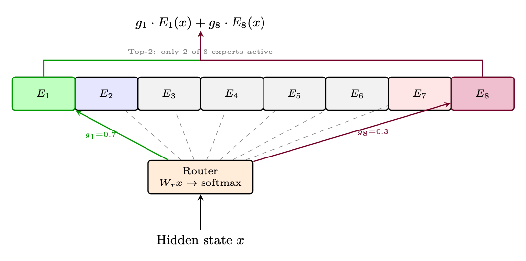
Figure 1.11: MoE layer with 8 experts and Top-2 routing. Only the two highest-gated experts are computed per token; the rest are skipped entirely.

1.10.2 Load Balancing

The Load Balancing Problem

Without constraints, the router may send most tokens to the same 1-2 experts ("expert collapse"). This wastes capacity and creates compute imbalance across GPUs (each expert typically lives on a different GPU). Solution: Add an auxiliary load-balancing loss:

N X

Lbal = α · N

i=1 fi · pi

where fi = fraction of tokens routed to expert i, pi = mean router probability for expert i. This encourages uniform expert utilization.

The core challenge in MoE is that top-k selection is not differentiable -- you can't backpropagate through a hard "pick the top 2" operation. The field has developed two key tricks to solve this:

The Routing Differentiability Problem

The router computes logits h(x) = Wr · x for each expert, then selects the top-k. But:

• The selected experts get gradients through their gate weights (softmax over selected)

• The selection decision itself (which k to pick) has zero gradient

• Without a trick, the router can get stuck: an expert never selected →never gets a gradient signal →never gets selected

Approach 1: Noisy Top-K Gating [105]. Add learnable Gaussian noise to the router logits before the top-k selection:

h(x) = Wg · x (clean logits)

H(x) = h(x) + ϵ · Softplus(Wnoise · x), ϵ ∼N(0, 1) (noisy logits)

( vi if vi is in the top k −∞ otherwise (1.11)

TopK(v, k)i =

g(x) = softmax �TopK(H(x), k) � (sparse gates)

• Wnoise is a learned noise magnitude -- the model learns how much exploration each expert needs

• During training, noise occasionally promotes "underdog" experts into the top-k, giving them gradient signal

• At inference, noise is removed: use clean logits h(x) for deterministic routing

• The Softplus ensures noise scale is always positive

Approach 2: Gumbel-Softmax Trick (for differentiable discrete sampling). An alternative from the variational inference literature [107]. The Gumbel-Max trick provides exact sampling from a categorical distribution:

z = arg max i [log πi + Gi] , Gi ∼Gumbel(0, 1) (1.12)

where Gumbel noise is generated as Gi = −log(−log(Ui)), Ui ∼Uniform(0, 1). For top-k routing: taking the top-k of (log πi + Gi) gives k samples without replacement from the categorical distribution defined by π. Since arg max is non-differentiable, the Gumbel-Softmax relaxation replaces it with a temperaturecontrolled softmax:

ˆgi = exp ((log πi + Gi)/τ) P j exp ((log πj + Gj)/τ) (1.13)

• τ →0: approaches a hard one-hot (exact but non-differentiable)

• τ →∞: approaches uniform (differentiable but uninformative)

• In practice, anneal τ from 1.0 down to 0.1-0.5 during training

• Straight-through estimator: use hard top-k in the forward pass, but Gumbel-Softmax gradients in the backward pass -- best of both worlds

• Sparsely-Gated MoE [105], Mixtral [106], DeepSeek-V2 [108]: Use Noisy Top-K with Gaussian noise. Simple, effective, well-proven at scale.

• Switch Transformer [109]: Simplified to Top-1 with no noise (relies on load-balancing loss alone).

• Research / smaller-scale MoE: Some use Gumbel-Softmax for fully differentiable routing, especially when learning the routing itself is the research objective.

• Key insight: Both approaches solve the same problem (making discrete selection trainable) via noise injection. Gaussian noise is simpler; Gumbel noise has stronger theoretical guarantees for categorical sampling.

1.10.4 Notable MoE Models

Model Total Params Active Params Experts Innovation

Switch Transformer [109] 1.6T 100B 128, Top-1 First large-scale MoE; simplified routing Mixtral 8x7B [106] 47B 13B 8, Top-2 Open-weight; matches Llama-2 70B quality DeepSeek-V2 [108] 236B 21B 160, Top-6 DeepSeekMoE with shared + routed experts Qwen-MoE [32] 14.3B 2.7B 60, Top-4 Fine-grained experts for efficiency DBRX [110] 132B 36B 16, Top-4 Fine-grained with 4 experts per block

1.11 Diversity in LLM Training

Diversity -- in training data, model outputs, and optimization trajectories -- is critical for preventing mode collapse and ensuring robust, general-purpose LLMs. This section covers the key diversity mechanisms applicable to all LLM training phases.

1.11.1 Sampling Diversity

Sampling Strategies for Diverse Generation

• Temperature τ: P(xi) ∝exp(logiti/τ). Higher τ = more uniform distribution = more diverse. Typical: τ = 0.7-1.0 for RLHF generation.

• Top-k: Only sample from the k highest-probability tokens. Prevents degenerate lowprobability tokens.

• Top-p (nucleus): Sample from the smallest set of tokens whose cumulative probability ≥p. Adaptive: more diverse when the model is uncertain.

• Min-p: Only keep tokens with P ≥pmin × Pmax. More principled than top-k.

• Frequency/presence penalty: Penalize tokens that appeared in the response. Encourages lexical diversity.

• Prompt diversity: Cover different domains, difficulty levels, and formats. The Goldilocks principle: prompts should have 20-80% success rate.

• Deduplication: Remove near-duplicate training examples (MinHash, n-gram overlap). Duplicates cause overfitting to specific patterns.

• Data mixing: Balance across tasks/domains using temperature-weighted sampling or curriculum strategies.

1.11.3 Diversity-Promoting Methods

Method How It Promotes Diversity

Temperature scaling Higher τ flattens the distribution; more tokens become plausible. Top-p / Min-p Adaptive thresholds allow wider sampling when the model is uncertain. Frequency penalty Penalizes repeated tokens, forcing lexical variety within a response. Data deduplication Removing near-duplicates from training data prevents overfitting to specific patterns. Multi-domain mixing Temperature-weighted sampling across domains ensures broad coverage. Verbalized sampling Prompt the model to explicitly verbalize a probability distribution over responses [111]. See §7.5.

1.12 Text Generation: Decoding Methods

A trained language model outputs a probability distribution over the vocabulary at each step: P(xt|x<t). The decoding strategy determines how we select the next token from this distribution. This choice profoundly affects output quality, diversity, and coherence.

1.12.1 Greedy Decoding

The simplest strategy: always pick the highest-probability token.

xt = arg max v∈V P(v|x<t)

Intuition: Like always taking the most obvious next word in a sentence. "The capital of France is..." →"Paris" (probability 0.92). Pros: Deterministic, fast, no hyperparameters.

Cons: Produces repetitive, generic text. Misses high-quality sequences where an early lowprobability token leads to a globally better output. No diversity.

1.12.2 Beam Search

Maintain B (beam width) partial hypotheses in parallel, expanding each by the top-k tokens and keeping the B highest-scoring complete sequences:

t X

score(y1:t) =

i=1 log P(yi|y<i)

With length normalization to avoid favoring short sequences:

|y| X

Cons: Still tends toward generic, repetitive text for open-ended generation; B× more compute; all beams often converge to similar outputs.

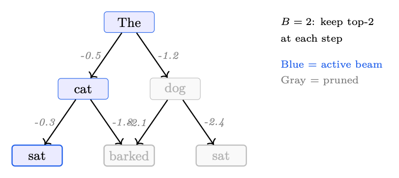
Figure 1.12: Beam search with B = 2. At each step, only the 2 highest-scoring partial sequences survive (blue). Lower-scoring alternatives are pruned (gray).

1.12.3 Diverse Beam Search

Standard beam search produces near-duplicate beams. Diverse beam search [112] partitions beams into G groups and adds a dissimilarity penalty between groups:

scoreg(yt) = log P(yt|y<t) −λ X

g′<g ∆(yt, Yg′)

where ∆measures overlap (e.g., Hamming diversity) with tokens already selected by earlier groups, and λ controls diversity strength. Intuition: Like forcing a brainstorming group to generate different ideas -- each subgroup is penalized for repeating what earlier subgroups said. Pros: Produces genuinely different candidate sequences; useful for reranking pipelines.

Cons: Diversity penalty can degrade individual beam quality; more hyperparameters (G, λ).

1.12.4 Top-k Sampling

Sample from only the k most probable tokens, redistributing probability mass:

  

P(v|x<t) P v′∈Top-k P(v′|x<t) if v ∈Top-k

P ′(v|x<t) =

 

0 otherwise

Intuition: After "The cat sat on the...", only consider the top k plausible continuations ("mat", "floor", "couch", ...) and ignore extremely unlikely ones ("quantum", "archipelago"). Pros: Removes tail noise; simple to implement.

Sample from the smallest set of tokens whose cumulative probability exceeds p:

(

)

S ⊆V : X

Top-p = min

v∈S P(v|x<t) ≥p

where tokens are sorted by descending probability and added until the threshold p is reached. Intuition: Adaptively resize the candidate pool. If the model is confident ("Paris" at 95%), the nucleus is tiny. If uncertain ("The movie was..."), the nucleus expands to include many plausible adjectives. Pros: Adapts to distribution shape; widely used default (p = 0.9-0.95).

Cons: Still includes some low-quality tokens at the tail of the nucleus; the threshold is a single global hyperparameter.

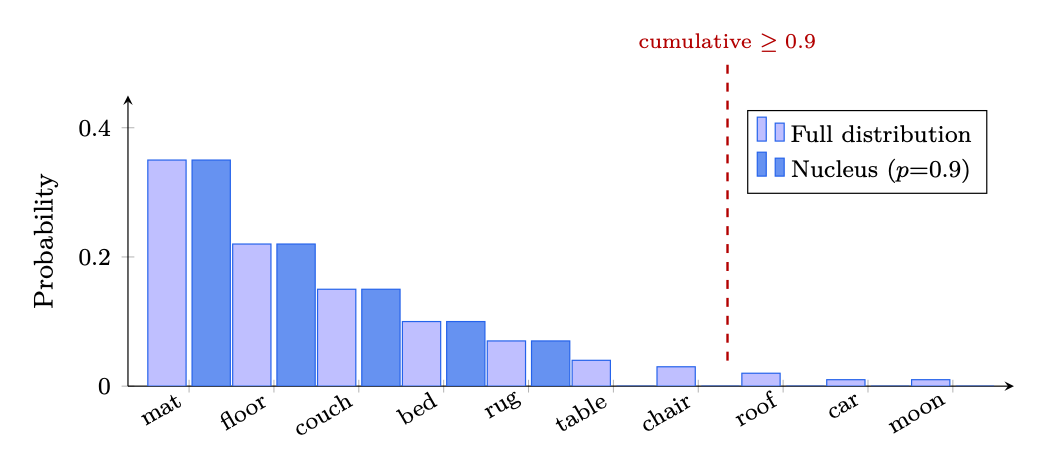
Figure 1.13: Top-p (nucleus) sampling: tokens are sorted by probability and included until cumulative mass reaches p = 0.9. The nucleus (dark blue) adapts its size to the distribution shape -- here 5 tokens suffice.

Top-kk vs. Top-pp

Consider predicting the next word:

• After "2 + 2 =": distribution is peaked -- top-1 token ("4") has 99% mass. Top-k=50 wastefully considers 49 wrong answers. Top-p=0.9 correctly picks just "4".

• After "I enjoy eating": distribution is flat -- many foods are plausible. Top-k=5 is too restrictive. Top-p=0.9 might include 50+ tokens, matching the actual uncertainty.

Top-p adapts; top-k doesn't. In practice, both are often combined: sample from top-p intersected with top-k.

1.12.6 Min-p Sampling

A recent alternative that sets a relative probability floor [113]:

Min-p = � v ∈V : P(v|x<t) ≥pmin · max v′ P(v′|x<t) �

Only tokens with probability at least pmin times the top token's probability are kept. Intuition: "Only consider tokens that are at least 10% as likely as the best token." If the top token has probability 0.8, only tokens above 0.08 survive. If the top token has probability 0.05 (very uncertain), tokens above 0.005 survive -- naturally expanding the pool. Pros: Scales naturally with model confidence; fewer degenerate samples than top-p on peaked distributions; single intuitive parameter.

1.12.7 Temperature Scaling

Before applying any sampling strategy, logits are divided by temperature T:

PT (v|x<t) = exp(zv/T) P v′ exp(zv′/T)

• T < 1: Sharpens distribution →more deterministic, focused outputs.

• T = 1: Unmodified model distribution.

• T > 1: Flattens distribution →more random, creative outputs.

• T →0: Becomes greedy decoding. T →∞: Becomes uniform sampling.

Common settings: T = 0.7 for factual tasks, T = 1.0-1.2 for creative writing, T = 0.0 (greedy) for code/math.

1.12.8 Contrastive Decoding

Contrastive decoding [114] exploits the difference between a strong model (expert) and a weak model (amateur) to amplify the expert's unique knowledge:

xt = arg max v∈V(x<t) [log Pexpert(v|x<t) −log Pamateur(v|x<t)]

where V(x<t) = {v : Pexpert(v|x<t) ≥α · maxv′ Pexpert(v′|x<t)} is an adaptive plausibility constraint. Intuition: The amateur model captures generic, obvious patterns (common words, repetition). Subtracting its log-probabilities removes this "generic signal," leaving the expert's distinctive knowledge and reasoning. Like removing background noise from a recording to hear the signal. Pros: Reduces repetition and generic phrasing; improves factuality and coherence without additional training; works with any model pair.

Cons: Requires running two models (2× compute); sensitive to amateur model choice; the plausibility threshold α needs tuning.

1.12.9 Repetition Penalties

Orthogonal to the sampling strategy, repetition penalties discourage the model from repeating tokens. Given the raw logit zv for token v (i.e., the unnormalized score output by the LM head before softmax), the penalized logit is:

( zv/θ if v ∈generated tokens and zv > 0 zv · θ if v ∈generated tokens and zv < 0

z′ v =

where θ > 1 is the penalty factor (typically 1.1-1.3). In both cases, the effect is to push the logit toward zero--reducing the probability of previously generated tokens. Frequency and presence penalties are simpler additive variants used by OpenAI APIs:

z′ v = zv −α · count(v) −β · 1[v ∈generated]

where α is the frequency penalty (proportional to how many times v appeared) and β is the presence penalty (flat penalty for any prior occurrence).

1.12.10 Practical Comparison

Method Deterministic Diversity Quality Best For

Greedy Yes None Medium Code, factual QA Beam Search (B=4-8) Yes Low High (narrow) Translation, summarization Diverse Beam Search Yes Medium High Candidate generation for reranking Top-k (k=50) No Medium Medium General-purpose generation Top-p (p=0.9) No Adaptive High Default for openended tasks Min-p (pmin=0.1) No Adaptive High Robust alternative to top-p Contrastive Yes Low Very High Factual, coherent long-form

Decoding in Practice: "Once upon a time"

Given the prompt "Once upon a time,":

• Greedy: "there was a young girl who lived in a small village..." (generic fairy tale)

• Top-p=0.9, T=1.0: "the rivers ran backwards and the fish learned to fly..." (creative, surprising)

• Top-p=0.9, T=0.3: "there was a kingdom ruled by a wise and just king..." (coherent, conventional)

• Contrastive: "in the amber-lit corridors of a collapsing star, two minds argued about the nature of time..." (distinctive, avoids clichés)

Same model, same prompt -- decoding strategy determines the character of the output.

1.12.11 Constrained Decoding (Structured Generation)

All methods above sample from the full vocabulary at each step. Constrained decoding restricts the set of allowed tokens so that the output is guaranteed to conform to a formal grammar--typically a JSON schema, regex, or context-free grammar (CFG).

Core mechanism. At each decoding step t, a token mask Mt ⊆V is computed from the current parser state. Only tokens in Mt receive their original logits; all others are set to −∞before softmax:

( P(v|x<t)/Z if v ∈Mt 0 otherwise

P ′(v|x<t) =

where Z = P v∈Mt P(v|x<t) renormalizes. Because the mask changes every step (it depends on what has been generated so far), the constraint is enforced incrementally--the model cannot produce an invalid prefix at any point.

From schema to mask. The compilation pipeline is:

JSON Schema compile −−−−→Regex compile −−−−→FSM (DFA) index −−−→Token Mask per State

Key libraries.

• Outlines [115]: Compiles JSON schemas and regexes into interleaved FSM-guided generation. Supports any model with a logits interface.

• lm-format-enforcer1: Similar FSM approach with a focus on integration with serving frameworks (vLLM, TGI).

• Guidance2 (Microsoft): Interleaves constrained generation with control flow (loops, conditions), enabling complex structured outputs beyond flat schemas.

• XGrammar [116]: Pushdown-automaton-based engine supporting full context-free grammars (not just regular languages), used in MLC-LLM and vLLM for grammar-mode decoding.

Trade-offs. Constrained decoding guarantees syntactic validity--no post-hoc parsing failures, no retries. However:

• Semantic quality: Forcing structure can degrade content quality if the model's probability mass for the "correct" answer lies outside the grammar. In practice this is rare for well-trained models on well-designed schemas.

• Compilation cost: The FSM index must be built per schema. For complex schemas this can take 1-5 s, but it is amortized over all requests using that schema.

• Grammar coverage: Regex/FSM handles JSON, YAML, SQL fragments, and most structured formats. Full CFGs (via XGrammar or LALR parsers) cover languages like Python or XML.

When to Use Constrained Decoding

Use constrained decoding whenever the consumer of the model's output is a program rather than a human. Tool-calling agents, API backends, and data-extraction pipelines all benefit from guaranteed valid structure. For free-form prose or creative text, unconstrained sampling remains appropriate.

1.13 Prompt Engineering

Prompt engineering is the discipline of designing inputs to LLMs that reliably elicit desired behaviour-- without changing model weights. While fine-tuning modifies the model, prompt engineering exploits the model's existing capabilities through careful framing, examples, and structure. It is the fastest, cheapest, and most accessible lever for improving LLM outputs, and remains essential even when using fine-tuned models.

1.13.1 In-Context Learning (ICL)

In-context learning [21] is the remarkable ability of large language models to learn tasks at inference time purely from examples provided in the prompt--with no gradient updates. The model implicitly infers the task from the pattern of input-output pairs and generalizes to new inputs.

Why In-Context Learning Works

• Implicit Bayesian inference: The model has seen millions of tasks during pretraining. The prompt examples locate the relevant task in the model's learned distribution [117].

• Task vectors: ICL creates implicit task representations in the residual stream that steer generation toward the demonstrated format and content [118].

Scaling behaviour. ICL emerges primarily in models above ∼1B parameters and improves loglinearly with model scale [21]. Smaller models can memorize examples but struggle to generalize to novel inputs within the same context window.

1.13.2 Zero-Shot Prompting

Zero-shot prompting provides no examples--only a task description or instruction. The model must rely entirely on its pretrained knowledge and instruction-tuning to produce the correct format and content.

Zero-Shot Classification

Classify the following movie review as POSITIVE or NEGATIVE.

Review: "The cinematography was breathtaking but the plot felt rushed and predictable."

Sentiment:

When zero-shot works well:

• Tasks the model has seen extensively during pretraining/SFT (translation, summarization, sentiment)

• Well-specified instructions with unambiguous output format

• Instruction-tuned models (e.g., ChatGPT, Claude, Llama-3-Instruct) significantly outperform base models at zero-shot tasks [9]

When zero-shot fails: Novel formats, domain-specific labeling schemes, or ambiguous tasks where the model cannot infer your exact requirements from the instruction alone.

1.13.3 Few-Shot Prompting

Few-shot prompting [21] provides k input-output examples ("shots") before the actual query. This is the most common form of in-context learning and remains one of the most effective prompting strategies.

Few-Shot Named Entity Recognition

Extract named entities from the text. Format: [ENTITY ]( TYPE)

Text: "Apple released the iPhone 15 in Cupertino." Entities: [Apple ](ORG), [iPhone 15]( PRODUCT), [Cupertino ](LOC)

Text: "Elon Musk announced Tesla 's new factory in Berlin." Entities: [Elon Musk ](PER), [Tesla ](ORG), [Berlin ](LOC)

Text: "OpenAI partnered with Microsoft to deploy GPT -4." Entities:

1. Diversity: Cover the range of expected inputs (different lengths, edge cases, categories).

2. Ordering: Place harder or more representative examples last (recency bias) [119].

3. Label balance: If classifying, include examples from all classes to avoid majority-class bias.

4. Format consistency: Every example must follow the exact same structure. The model mimics the pattern.

5. Relevance: Use examples semantically similar to the target query for best results [120].

How many shots? Performance typically improves from 0 to 4-8 examples, then plateaus. Beyond ∼20 examples, gains are marginal and you risk filling the context window. Min et al. [121] showed that the format and label space of examples matter more than label correctness--even random labels help (though correct labels help more).

1.13.4 Instruction-Following Prompts

Instruction-tuned models respond best to clear, structured instructions. The key insight: treat the prompt as a specification, not a suggestion.

Anatomy of an Effective Instruction Prompt

1. Role/Persona: Define who the model is ("You are a senior data scientist...")

2. Task: What to do, stated clearly and unambiguously

3. Context: Background information the model needs

4. Constraints: Length limits, tone, what to avoid, output format

5. Examples (optional): Show the desired output format

6. Input: The actual data to process

Instruction Prompt with Constraints

Role: You are a medical literature reviewer.

Task: Summarize the following research abstract for a general audience.

Constraints: - Maximum 3 sentences - No jargon (explain any technical terms) - Include the key finding and its clinical implication - Do NOT speculate beyond what the abstract states

Abstract: [...]

System prompts vs. user prompts. Modern chat APIs separate the system prompt (persistent instructions, role definition) from the user message (per-turn input). System prompts are processed with higher attention priority in most models and provide a natural place for role definitions, constraints, and output format specifications [23].

1.13.5 Structured Output Prompts (JSON/XML)

Extract the following information from the customer email. Respond ONLY with valid JSON , no other text.

Schema: {

"intent": "refund|complaint|question|praise", "urgency": "low|medium|high", " product_mentioned ": "string or null", "summary": "one sentence summary" }

Email: [...]

Techniques for reliable structured output:

• Schema-first: Show the exact JSON schema before the input. The model treats it as a template.

• Constrained decoding: Use grammar-based sampling (e.g., Outlines [115], Guidance) to guarantee syntactically valid JSON at the token level.

• XML tags: For nested or multi-part outputs, XML tags (e.g., <thinking>...</thinking>) provide unambiguous delimiters that models follow reliably.

• Pydantic/TypeScript types: Providing type definitions helps models understand field constraints (OpenAI's function calling uses JSON Schema internally).

JSON in Prompts -- Common Pitfalls

• Models may add markdown fences ("'json ... "') -- instruct explicitly to output raw JSON.

• Nested objects and arrays increase hallucination risk -- flatten schemas where possible.

• Enum fields (fixed choices) are much more reliable than free-text fields.

• Always validate outputs programmatically; no prompt guarantees 100% compliance without constrained decoding.

JSON Prompting: Structuring the Input. A distinct but complementary technique is JSON prompting--formatting the prompt itself as JSON rather than natural language. This exploits the model's extensive pre-training on structured data (APIs, configs, code) to improve instruction adherence, reduce ambiguity, and enable deterministic parsing of multi-field requests.

JSON Prompting with System Prompt

=== SYSTEM === You are a senior code reviewer. Analyze code for bugs , security issues , and style violations. Always respond in the JSON schema provided.

=== USER (JSON prompt) === {

"task": "code_review", "language": "python", " severity_filter ": "high", "code": "def login(user , pw):\n query = ...", " output_schema": {

"issues": [{

"line": "int",

Why JSON prompting works:

• Unambiguous field boundaries: No confusion about where one instruction ends and another begins.

• Typed constraints: Fields like "severity_filter": "high" are clearer than "only show high severity issues."

• Schema-as-contract: Including output_schema in the input mirrors API design patterns the model has seen extensively during pre-training.

• System prompt still essential: The system message provides role, tone, and behavioral constraints that don't fit naturally in a JSON payload.

1.13.6 Chain-of-Thought (CoT) Prompting

Chain-of-thought prompting [122] asks the model to produce intermediate reasoning steps before giving a final answer. This simple technique dramatically improves performance on tasks requiring multi-step reasoning: arithmetic, logic, commonsense inference, and code generation.

Why CoT works:

• Serializes computation: Transformers have fixed depth but variable-length generation. CoT converts parallel (hard) problems into sequential (easy) steps, effectively increasing the model's computational budget.

• Reduces compounding errors: Each step is a simpler sub-problem with lower per-step error rate.

• Exposes intermediate state: Makes reasoning auditable and debuggable.

Chain-of-Thought Variants

Method Description

Zero-shot CoT [123] Append "Let's think step by step" to any prompt Few-shot CoT [122] Provide examples with explicit reasoning chains Self-Consistency [124] Sample N CoT paths; majority-vote the final answer Tree of Thoughts [125] Explore multiple reasoning branches with backtracking Plan-and-Solve [126] First plan the steps; then execute each step ReAct [127] Interleave Reasoning and Acting (tool use)

Zero-Shot Chain-of-Thought

Q: A store has 45 apples. They sell 3/5 of them in the morning and 1/3 of the remaining in the afternoon. How many apples are left?

Let's think step by step.

A: Morning sales: 45 * 3/5 = 27 apples sold. Remaining after morning: 45 - 27 = 18.

Self-Consistency. Wang et al. [124] showed that sampling multiple chain-of-thought reasoning paths and taking a majority vote over final answers significantly outperforms single-path CoT. The intuition: correct reasoning paths tend to converge on the same answer, while errors are typically idiosyncratic. This trades compute (generating N samples) for accuracy--practical when latency is less important than correctness.

When CoT hurts. CoT is not universally beneficial. For simple tasks (single-step classification, retrieval, formatting), CoT adds unnecessary tokens, increases latency, and can even introduce errors through overthinking. Use CoT selectively for tasks where you expect multi-step reasoning to be required.

1.13.7 Advanced Prompting Techniques

Retrieval-Augmented Generation (RAG). Rather than relying solely on the model's parametric memory, RAG [128] retrieves relevant documents and includes them in the prompt:

Context (retrieved): [document chunks] Question: [user query] Answer based ONLY on the provided context.

This grounds the model's responses in verifiable sources and dramatically reduces hallucinations for knowledge-intensive tasks.

Prompt Chaining and Decomposition. Complex tasks benefit from being broken into a pipeline of simpler prompts, where the output of one becomes the input to the next:

1. Extract key facts from document

2. Reason over extracted facts

3. Format final answer

Each step can use a different prompt template, model, or temperature setting. This is more controllable than a single monolithic prompt and enables targeted debugging.

Constitutional AI / Self-Critique. Bai et al. [129] introduce prompts that ask the model to critique and revise its own output against a set of principles:

[Generate initial response] Critique: Does this response violate any of the following principles? [list principles] Revision: Rewrite the response addressing the critique.

Meta-Prompting and Prompt Optimization. Rather than hand-crafting prompts, recent work automates prompt design:

• APE [130]: Uses an LLM to generate and score candidate prompts automatically.

• DSPy [131]: Compiles declarative task descriptions into optimized prompt pipelines with learned few-shot examples.

1. Query decomposition: Break the user question into atomic sub-questions that each target a narrow aspect.

2. Attentive retrieval: For each sub-query, retrieve or highlight only the relevant context slice--forcing the model to attend to it.

3. Aggregation: Combine sub-answers into a coherent final response.

This is particularly effective for long-document QA, multi-hop reasoning over large retrieval sets, and agentic tasks where the context window contains many tool outputs. ARQ can be seen as a structured form of chain-of-thought that explicitly manages where the model looks, not just how it reasons.

1.13.8 Best Practices: Crafting Effective Prompts

Based on empirical findings across the literature and practitioner experience, the following principles reliably improve prompt quality:

The Prompt Engineering Checklist

1. Be specific and unambiguous: Replace "summarize this" with "summarize in 2-3 bullet points, each under 20 words, focusing on actionable findings."

2. Show, don't tell: One good example is worth 100 words of instruction. When in doubt, add a few-shot example.

3. Define the output format explicitly: Specify JSON schema, bullet points, table format, or exact delimiters. Never leave format to interpretation.

4. Use delimiters for input data: Wrap user inputs in clear delimiters (""", <input>...</input>, --) to separate instructions from data.

5. Assign a role: "You are a [domain expert] who [specific behaviour]" primes relevant knowledge and tone.

6. Specify what NOT to do: Negative constraints ("do not explain your reasoning", "never output more than 5 items") are often more effective than positive ones.

7. Add chain-of-thought for reasoning tasks: Append "Think step by step" or provide worked examples for math, logic, or multi-hop questions.

8. Control temperature appropriately: Use T ≈0 for factual/deterministic tasks; T ≈0.71.0 for creative/diverse outputs.

9. Iterate empirically: Treat prompts as code--version them, A/B test them, and measure performance on representative eval sets.

10. Leverage recency bias: Place the most critical instructions and examples at the end of the prompt (closest to the generation point).

The Prompt Engineering Mindset

Think of prompt engineering as programming in natural language. The model is a powerful but literal interpreter--it will do exactly what you ask, interpreted in the most likely way given its training distribution. Common principles from software engineering apply:

Failure Mode Symptom Solution

Instruction amnesia Model ignores constraints in long prompts Move constraints to end; repeat key rules; use system prompt Format drift Output starts correct but degrades over long generations Use constrained decoding; break into shorter chained prompts Sycophancy Model agrees with incorrect premises in the prompt Add "challenge assumptions if incorrect"; use system-level instruction Hallucinated details Model invents facts not in provided context Add "if unknown, say I don't know"; use RAG with source attribution Refusal over-triggering Model refuses benign requests due to safety training Rephrase to clarify legitimate intent; provide explicit context for why the request is appropriate

• DRY (Don't Repeat Yourself): Unless fighting attention decay in long contexts

• Separation of concerns: Different prompt sections for role, constraints, examples, and input

• Test-driven development: Define expected outputs before writing the prompt

• Version control: Track prompt iterations and their eval scores

• Modularity: Build reusable prompt templates; parameterize variable parts

When prompting fails to achieve the desired quality after systematic iteration, that is the signal to move to fine-tuning (SFT) or reinforcement learning (RLHF/DPO).

1.14 Model Compression Methods

Model compression reduces model size and inference cost while preserving quality. Three main approaches: quantization (reduce precision), pruning (remove parameters), and distillation (train a smaller model to mimic a larger one).

1.14.1 Quantization

Quantization reduces model size and inference cost by representing weights (and optionally activations) in lower-precision formats. The core trade-off is compression ratio versus quality degradation.

Quantization Overview

Quantization reduces the numerical precision of model weights (and optionally activations) from FP32/BF16 to lower-bit formats:

xq = round �x −z

� , xdequant = s · xq + z

s

where s is the scale factor and z is the zero-point.

When to Quantize

• Inference serving: Always quantize. W4A16 (4-bit weights, BF16 activations) is the sweet spot -- 2× memory savings, <1% quality loss for 70B+ models.

• Training: FP8 on H100 gives 2× throughput with minimal quality loss. BF16 is still the default for smaller models.

• Edge deployment: GGUF Q4_K_M for local inference on consumer hardware.

Method Bits Type Key Idea

GPTQ [134] 4-bit PTQ, weight-only Layer-wise quantization minimizing ∥WX −ˆWX∥2 via optimal brain surgeon. AWQ [135] 4-bit PTQ, weight-only Protects salient weights (those with large activations). 1% of weights carry 99% importance. GGUF [136] 2-8 bit PTQ, weight-only CPU-optimized format (llama.cpp). Per-block quantization with multiple types. FP8 (E4M3) 8-bit Training + inference Native H100 support. 2× throughput vs BF16. SmoothQuant [137] W8A8 PTQ, weight+act. Smooths activation outliers into weights before quantization. Enables INT8 GEMM. QAT [138] 4-bit QAT Trains with simulated quantization. Highest quality but expensive. AQLM [139] 2-bit PTQ, additive codes Extreme compression via learned additive quantization codebooks.

• RLHF: Quantize the frozen models (reference, reward model) to INT8/FP8. Keep the policy in BF16 for training precision.

1.14.2 Pruning

Why Prune? Modern LLMs contain billions of parameters, yet empirical studies consistently show that a large fraction of these weights contribute minimally to model outputs. Pruning exploits this over-parameterization: by removing redundant weights, we reduce memory footprint (enabling deployment on smaller GPUs or edge devices), inference latency (fewer multiply-accumulate operations per forward pass), and serving cost (higher throughput per dollar). Unlike quantization, which reduces the precision of all weights uniformly, pruning selectively eliminates weights--enabling multiplicative savings when combined with quantization (e.g., a 50% sparse, 4-bit model uses 4× less memory than the dense BF16 baseline). The challenge is achieving high sparsity without degrading generation quality, which has driven the development of principled one-shot methods that require no retraining.

Pruning Methods

• Unstructured pruning: Zero out individual weights below a threshold. High sparsity (50-90%) possible. Requires sparse GEMM kernels (2:4 on A100/H100).

• Structured pruning: Remove entire attention heads, layers, or FFN neurons. Directly reduces FLOPS without specialized kernels.

• SparseGPT [140]: One-shot pruning using approximate inverse Hessian. 50% unstructured sparsity with minimal quality loss on 175B models.

• Wanda [141]: Prune by |w| × ∥x∥(weight magnitude times input activation norm). No calibration data needed. Competitive with SparseGPT.

NVIDIA 2:4 Structured Sparsity

A100/H100 Tensor Cores natively support 2:4 sparsity: out of every 4 elements, at most 2 are non-zero. This gives exactly 2× speedup on supported operations with hardware acceleration. The constraint: you must achieve exactly 50% sparsity in this specific pattern, which limits flexibility compared to arbitrary sparsity.

Knowledge distillation [142] transfers the learned behaviour of a large teacher model into a smaller, cheaper student model. The core idea is that the teacher's output distribution over tokens carries far richer signal than ground-truth hard labels alone -- revealing inter-class similarities, calibration, and uncertainty that the student can exploit.

Temperature-Scaled Softmax. To expose the "dark knowledge" in the teacher's logits we soften the distribution with a temperature T > 1:

p(T) i = exp(zi/T) P j exp(zj/T)

At high temperature the probability mass spreads across more tokens, making near-miss alternatives visible. During training the same temperature is applied to the student; at inference the student uses T = 1.

General Distillation Loss.

Ldistill = α T 2 · KL �P (T) teacher ∥P (T) student � + (1 −α) · LCE(y, P (1) student)

The T 2 factor compensates for the reduced gradient magnitude of softened distributions. Typical values: T ∈[2, 20], α ∈[0.5, 0.9] (more weight on KL when teacher quality is high).

Table 1.18: Knowledge distillation paradigms for LLMs.

Paradigm Mechanism Pros Cons

Offline / White-box Teacher logits precomputed; student trains on full distributions

Full distribution signal; one-time teacher cost

Stale data; storage heavy

Adapts to student weaknesses 2× compute; complex infra

Online / Co-training Teacher generates onthe-fly; student sees fresh logits

Black-box (API) Only teacher text outputs available (no logits)

Works with proprietary models Loses dark knowledge; SFT-like

Self-distillation Model distills into a smaller version of itself

No separate teacher needed Teacher = student family; ceiling

Offline (White-Box) Distillation. The teacher's full logit vector (or top-k logits for storage efficiency) is recorded for each training token. The student minimises the KL divergence against these stored distributions. This is the most data-efficient paradigm when teacher access is unrestricted. Motivation: Decouple teacher inference from student training -- run the teacher once on high-end hardware, then train many students cheaply. Pros: Deterministic, reproducible; teacher cost is amortised; full distributional signal.

Cons: Requires storing |V |-dimensional vectors per token (mitigated by top-k pruning); teacher cannot adapt to student failures.

Cons: Double the GPU cost; synchronisation complexity; harder to scale.

Black-Box (API) Distillation. When only text outputs are available (e.g. distilling from a proprietary API), the student is trained via SFT on the teacher's generations, optionally augmented with chain-of-thought traces. Motivation: Practical reality -- most frontier models do not expose logits. Pros: Simple pipeline; works with any model behind an API.

Cons: No soft-label signal; prone to hallucination amplification; effectively supervised fine-tuning.

Self-Distillation. A model distils from a larger version within the same architecture family (e.g. Llama-3 70B →8B) or from its own checkpoints during training. Motivation: Avoid training a separate teacher; leverage the model's own capacity at different scales. Pros: Architecture compatibility; no external dependency.

Cons: Teacher ceiling equals model ceiling; cannot introduce genuinely new knowledge.

Dark Knowledge

Consider a language model predicting the next word after "The capital of France is". Hard labels say only "Paris" is correct. But the teacher's soft distribution might assign 5% to "Lyon", 2% to "Marseille", and near-zero to "banana" -- telling the student which errors are reasonable, which dramatically improves calibration and generalisation.

Practical Considerations for LLM Distillation.

• Sequence-level vs. token-level: Token-level KL is standard; sequence-level distillation (minimising KL over full sequences) better captures long-range coherence but is harder to optimise.

• Layer-wise hints: Matching intermediate representations (attention maps, hidden states) provides additional learning signal -- especially useful when student architecture differs.

• Data selection: Distillation data quality matters; curating diverse, hard examples yields better students than random sampling.

• Student capacity: Diminishing returns below ∼10% of teacher parameters; at extreme compression, architecture changes (e.g. MoE →dense) may be needed.

• Combining with quantization: Distillation + 4-bit quantization (e.g. QLoRA-distilled models) achieves near-teacher quality at 20× compression.

Method Size Speed Quality Use Case

BF16 (baseline) 140 GB 1× 100% Training, reference FP8 (E4M3) 70 GB 2× 99.5% H100 inference INT8 (SmoothQuant) 70 GB 1.8× 99% A100 inference 4-bit (AWQ) 35 GB 2.5× 97-98% Serving at scale 2-bit (AQLM) 17.5 GB 3× 90-93% Edge, experimental Pruned 50% (2:4) 70 GB 1.8× 97% Structured speedup Distilled 8B 16 GB 10× 80-85% Mobile, edge

1.15 Speculative Decoding Methods

Speculative decoding [143] accelerates autoregressive generation by predicting multiple tokens simultaneously, then verifying them in a single forward pass of the target model. It produces identical output distribution to standard decoding (no quality loss) while achieving 2-3× speedup.

1.15.1 Core Principle

Speculative Decoding Framework

1. A fast draft mechanism proposes k candidate tokens: ˆx1, . . . , ˆxk

2. The large target model runs a single forward pass on all k tokens (batched)

3. Verification: Accept tokens left-to-right while Ptarget(ˆxi) ≥ri·Pdraft(ˆxi) (where ri ∼U[0, 1])

4. On first rejection at position j: resample xj from an adjusted distribution, discard ˆxj+1, . . . , ˆxk

Key property: This acceptance/rejection scheme guarantees the final distribution equals Ptarget exactly. Speedup: If acceptance rate is α, expected tokens per step = 1−αk+1

1−α . At α = 0.8, k = 5: expected 3.4 tokens/step vs. 1 for standard decoding.

1.15.2 Methods Comparison

1.15.3 Medusa: Multi-Head Speculative Decoding

How Medusa Works Medusa adds k additional "prediction heads" to the LLM (sharing the same backbone):

• Head 0 (original): predicts token at position t + 1 (standard next-token)

• Head 1: predicts token at position t + 2 (skipping one)

• Head i: predicts token at position t + i + 1

• All heads run in parallel during a single forward pass

• A tree-structured verification validates multiple candidate sequences simultaneously

Method Draft Source Speedup Key Idea

Standard [143] Small model (1-7B) 2-3× Separate draft model generates candidates. Simple but requires loading 2 models. Medusa [144] Parallel LM heads 2-3× Add k extra prediction heads to the target model. Each predicts token at position +1, +2, . . . , +k. Eagle [145] Feature-level 2.5-3.5× Lightweight decoder generates draft tokens from target model's hidden states. Higher acceptance than Medusa. Eagle-2 [145] Context-aware 3-4× Dynamic draft tree with confidencebased expansion. State-of-the-art acceptance rates. N-gram Lookup N-gram cache 1.5-2× Match prompt n-grams against previously generated text. Zero cost; great for repetitive outputs. Lookahead [146] Jacobi iteration 2-2.5× Parallel Jacobi decoding with ngram verification. No draft model; uses target model itself. Multi-token [147] Modified arch. 2-3× Train the model to natively predict multiple tokens per step (Meta's approach in Llama).

Advantage: No separate draft model; heads are tiny (one linear layer each). Memory overhead: <1%.

1.15.4 Eagle: Feature-Level Drafting

Why Eagle Outperforms Medusa

Medusa's heads predict independently at each position -- they cannot condition on their own previous predictions (token at t + 2 doesn't know what was predicted at t + 1). Eagle fixes this with a lightweight autoregressive decoder that operates on the target model's hidden states:

1. Extract hidden states from the target model's last layer

2. Feed into a small (1-layer) decoder that autoregressively generates draft tokens conditioned on previous hidden states

3. This captures inter-token dependencies that Medusa misses

Result: Eagle achieves 85-95% acceptance rate vs. Medusa's 60-80%.

1.15.5 N-gram Speculative Decoding

N-gram Lookup Method

The simplest speculative decoding -- requires no additional model or training:

1. Maintain a cache of n-grams from the prompt and previously generated text

2. At each step, check if the current context's last n −1 tokens match any cached n-gram

3. If yes: propose the continuation as draft tokens

Best for: Code generation (repetitive patterns), structured outputs (JSON/XML), and prompts with repeated elements. Cost: Essentially zero.

from vllm import LLM , SamplingParams

# Standard speculative decoding (separate draft model) llm = LLM(

model="meta -llama/Llama -3-70B", tensor_parallel_size =4, speculative_config ={

"model": "meta -llama/Llama -3-8B", " num_speculative_tokens ": 5, }, )

# N-gram speculation (zero -cost , no draft model needed) llm = LLM(

model="meta -llama/Llama -3-70B", speculative_config ={

"method": "ngram", " num_speculative_tokens ": 5, " prompt_lookup_max ": 4, # Match up to 4-grams from prompt }, )

# EAGLE -style (feature -level draft , high acceptance rate) llm = LLM(

model="meta -llama/Meta -Llama -3-8B-Instruct", tensor_parallel_size =4, speculative_config ={

"model": "yuhuili/EAGLE -LLaMA3 -Instruct -8B", " num_speculative_tokens ": 2, "method": "eagle", " draft_tensor_parallel_size ": 1, }, )

# MLP speculator (IBM -style , lightweight head) llm = LLM(

model="meta -llama/Meta -Llama -3.1 -70B-Instruct", tensor_parallel_size =4, speculative_config ={

"model": "ibm -ai -platform/llama3 -70b-accelerator", " draft_tensor_parallel_size ": 1, }, )

When NOT to Use Speculative Decoding

• High batch sizes: At batch ≥64, generation is already compute-efficient. Speculation adds overhead (draft generation + verification) that doesn't pay off.

• Very different distributions: If draft model is too dissimilar to target, acceptance rate drops below 50% and speculation is slower than standard decoding.

• Short outputs: For <20 token outputs, the setup cost of speculation exceeds savings.

• Rule of thumb: Speculation helps most for latency-sensitive, single-stream generation (chatbots, interactive code completion).

LLMs generate fluent text that may be factually incorrect--a phenomenon called hallucination [148]. This section covers basic detection methods at the model level (without external retrieval or multiagent verification).

1.16.1 Types of Hallucination

Hallucination Taxonomy

• Intrinsic: Contradicts the provided input/context (e.g., summary says the opposite of the source)

• Extrinsic: Generates claims that cannot be verified from the input and are factually wrong

• Faithfulness: Output diverges from the instruction or specified constraints

1.16.2 Detection Methods (Model-Level)

Table 1.20: Basic hallucination detection methods that operate at the model level.

Method Mechanism Signal

Token-level entropy High entropy at generation time indicates uncertainty [149] H(P(xt)) > τ

1 T P t log P(xt)

Sequence log-prob Low average log-probability of the output suggests confabulation

Consistency sampling Generate N responses; low agreement = likely hallucination [150] Contradiction rate

Semantic entropy Cluster meanings (not strings); high semantic entropy = uncertain [151] Cluster diversity

DoLA Contrast logits between later vs. earlier layers; amplifies factual knowledge [152] Layer divergence

Semantic Entropy. Kuhn et al. [151] observe that token-level entropy is unreliable (paraphrases have different tokens but same meaning). Instead, they generate multiple responses, cluster them by semantic equivalence (via NLI), and compute entropy over meaning clusters:

SE = − X

c∈clusters P(c) log P(c)

High SE means the model produces semantically different answers--a strong hallucination signal.

SelfCheckGPT. Manakul et al. [150] detect hallucinations by checking self-consistency: generate multiple responses and verify whether claims in the main response are supported by the alternatives. If the model "disagrees with itself," the claim is likely hallucinated. No external knowledge needed.

DoLA (Decoding by Contrasting Layers). Chuang et al. [152] observe that factual knowledge emerges in later transformer layers while earlier layers retain more generic/uncertain representations. DoLA contrasts the logit distributions between a later ("mature") layer and an earlier ("premature") layer at each decoding step:

DoLA(xt) = softmax �log Plate(xt) −log Pearly(xt) �

1.17 LLM Safety and Responsible AI

Safety is not an afterthought--it is an integral part of the LLM training pipeline. This section covers the key dimensions of LLM safety and the mechanisms used to enforce responsible behavior.

1.17.1 Threat Taxonomy

Table 1.21: LLM safety threat categories.

Category Description and Examples

Harmful content Generating toxic, violent, or illegal instructions (bioweapons, CSAM) Bias and discrimination Perpetuating stereotypes; unfair treatment across demographics [153] Privacy violations Leaking PII from training data; memorization attacks [154] Jailbreaking Adversarial prompts that bypass safety guardrails [155] Misinformation Generating convincing but false claims (hallucination at scale) Dual-use Legitimate capabilities (coding, chemistry) weaponized for harm

1.17.2 Safety Training Pipeline

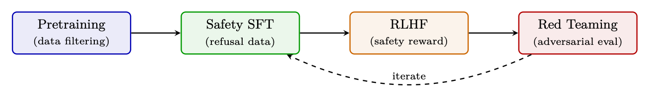
Figure 1.14: Safety is applied at every stage: data filtering in pretraining, refusal examples in SFT, safetyspecific reward models in RLHF, and iterative red-teaming.

1.17.3 Key Safety Mechanisms

Safety Techniques

• Data filtering: Remove toxic, biased, and PII-containing text from pretraining corpora

• Safety SFT: Train on examples of appropriate refusals ("I can't help with that because. . . ")

• Constitutional AI [129]: Self-critique using principles; model revises its own outputs against a constitution of rules

• Safety reward model: Separate RM trained on safety-annotated pairs; combined with helpfulness RM during RLHF via weighted sum

• Guardrails: Input/output classifiers that block harmful requests/responses at serving time

Balancing Helpfulness and Safety

Over-optimizing for safety creates an over-refusal problem: the model declines benign requests (e.g., refusing to discuss historical violence in an educational context). The goal is a Pareto-optimal policy that is maximally helpful within safety constraints:

max θ E[Rhelpful] subject to E[Rsafety] ≥τ

In practice, this is implemented as a weighted reward: R = αRhelpful + (1 −α)Rsafety with careful tuning of α (typically 0.6-0.8). Meta's Llama-3 reports using distinct safety and helpfulness reward models with margin-based weighting [25].

1.17.5 Evaluation

• Safety benchmarks: ToxiGen, RealToxicityPrompts, BBQ (bias), CrowS-Pairs

• Jailbreak robustness: GCG attacks [155], multi-turn jailbreaks, encoded prompts

• Over-refusal rate: Measure false-positive refusals on benign prompts (target <5%)

• Red team evaluations: Human adversarial testing with domain experts (biosecurity, cybersecurity)

Safety Is Never Complete

No combination of techniques provides absolute safety. New attack vectors are discovered continuously (multi-modal jailbreaks, fine-tuning attacks that remove safety training, many-shot prompting). Safety requires ongoing monitoring, rapid response to new threats, and defense-indepth (multiple independent layers).

Chapter 2