RL for Large Reasoning Models

RL for Large Reasoning Models

The emergence of large reasoning models represents one of the most significant developments in modern AI. Unlike standard language model training, which optimizes for next-token prediction, reasoning-focused RL teaches models to think before answering--allocating additional computation at inference time to explore, verify, and refine intermediate steps. This section provides a comprehensive technical treatment of the methods, architectures, and scaling laws that underpin this paradigm.

13.1 Motivation and Background

13.1.1 Why Reasoning Requires Different RL Approaches

Standard RLHF (Section 4.3) optimizes a single scalar reward over a complete response. For tasks requiring multi-step reasoning--mathematics, formal verification, competitive programming, scientific derivation--this formulation is insufficient for several reasons:

• Sparse rewards: A math problem may require 20 intermediate steps; a single outcome reward provides no gradient signal for the intermediate steps that led to an error.

• Long horizons: Reasoning chains can span hundreds to thousands of tokens, creating severe credit assignment problems.

• Combinatorial search: The space of valid reasoning paths is exponentially large; the model must learn to search this space efficiently.

• Verifiability: Unlike subjective text quality, mathematical and logical correctness is objectively verifiable, enabling automated reward computation without human annotation.

Key Insight: Reasoning as a Search Problem

Multi-step reasoning can be framed as a search problem over a tree of partial solutions. Each node in the tree is a reasoning state (prefix of the chain-of-thought), each edge is a reasoning step (a token or sentence), and the leaves are final answers. RL for reasoning teaches the model to navigate this tree efficiently--exploring promising branches, backtracking from dead ends, and allocating compute where it matters most.

13.1.2 Chain-of-Thought: Emergent Behavior vs. Trained Capability

• Trained CoT via RL produces models that intrinsically generate reasoning chains as part of their generation process, independent of prompting style. These chains are longer, more exploratory, and exhibit qualitatively different behaviors (self-correction, backtracking, verification).

The "Aha Moment" Phenomenon (DeepSeek-AI et al. 2025)

During RL training of reasoning models, researchers at DeepSeek observed a striking emergent behavior: at a certain point in training, models spontaneously began to reconsider their initial approaches mid-chain, using phrases like "Wait, let me reconsider. . . " or "Actually, I think I made an error. . . ". This self-correction behavior--which was not explicitly trained--emerged purely from the RL objective of maximizing final-answer accuracy. It suggests that RL can discover meta-cognitive strategies that are instrumentally useful for solving hard problems.

13.1.3 Test-Time Compute Scaling Laws

A central empirical finding motivating reasoning model research is that test-time compute scales predictably with performance. Let Ctrain denote training compute (FLOPs) and Ctest denote inference compute (tokens generated). The key observation is:

Accuracy(Ctrain, Ctest) ≈f(α log Ctrain + β log Ctest) (13.1)

for some monotone function f and constants α, β > 0. This implies that a smaller model with more inference compute can match a larger model with less inference compute--a fundamental shift in the compute-performance tradeoff.

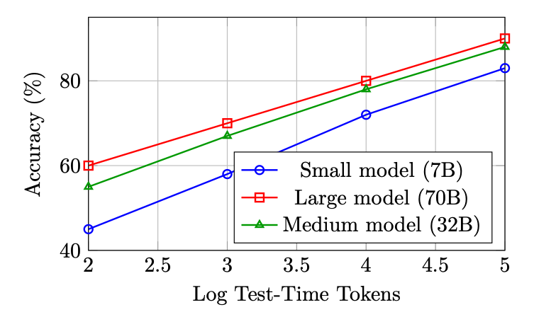
Figure 13.1: Schematic test-time compute scaling curves. Performance improves log-linearly with inference tokens across model sizes, and smaller models with more compute can approach larger models with less compute.

The scaling laws above show that investing more compute at inference can dramatically improve reasoning performance. This section provides a comprehensive treatment of the methods that operationalize test-time scaling -- from simple chain-of-thought to sophisticated tree and graph search algorithms. These methods form a spectrum trading inference cost for accuracy, and understanding their structure is essential for designing modern reasoning systems.

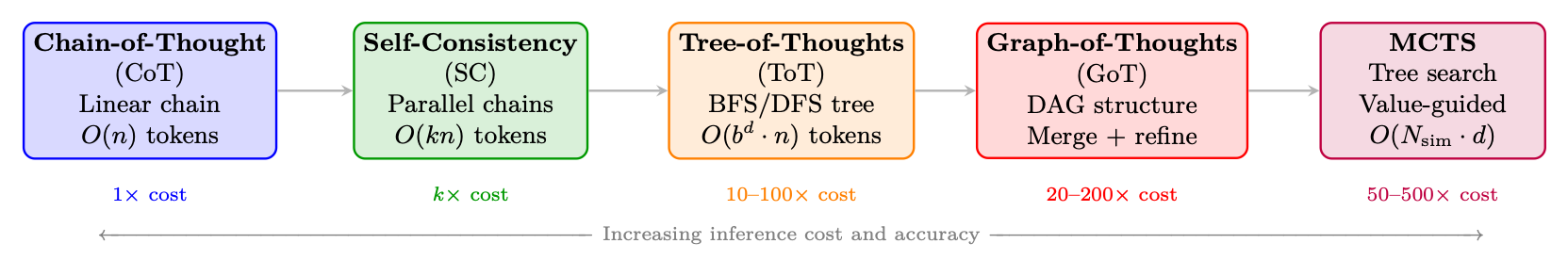
Figure 13.2: Spectrum of test-time scaling methods. Each method trades additional inference compute for improved reasoning accuracy. Methods build on each other conceptually: CoT introduces explicit reasoning, Self-Consistency adds sampling, ToT adds structured search, GoT adds merging operations, and MCTS adds learned value guidance.

13.2.1 Chain-of-Thought (CoT)

Chain-of-Thought prompting [122] is the foundation of all test-time scaling methods. Rather than directly outputting an answer, the model generates intermediate reasoning steps that decompose complex problems into manageable sub-problems.

Zero-Shot CoT. Kojima et al. [123] demonstrated that appending "Let's think step by step" to a prompt elicits reasoning behavior without any exemplars. This simple trigger activates latent reasoning capabilities in sufficiently large models (≥100B parameters).

Few-Shot CoT. Wei et al. [122] showed that providing a few exemplars with explicit reasoning traces enables smaller models to reason effectively:

Prompt = [(x1, z1, y1), (x2, z2, y2), . . . , (xk, zk, yk), (xtest, ?)] (13.2)

where zi are hand-written reasoning traces for exemplar (xi, yi).

Formal characterization. CoT converts a single-step prediction p(y|x) into a multi-step sequential generation: p(y|x) = X

z p(y|x, z) · p(z|x) ≈p(y|x, z∗) · p(z∗|x) (13.3)

where z∗= (z1, z2, . . . , zT ) is the greedy reasoning chain. The summation over all possible chains is intractable; standard CoT uses a single sample (greedy or temperature sampling).

Limitations. Single-chain CoT is fragile: if an early reasoning step is wrong, all subsequent steps build on a flawed foundation with no mechanism for recovery.

13.2.2 Self-Consistency (Majority Voting)

Self-Consistency [124] addresses CoT's single-chain fragility by sampling multiple independent reasoning chains and taking a majority vote over the final answers:

N X

ˆy = arg max y

i=1 1[yi = y], where (zi, yi) ∼p(·|x), T > 0 (13.4)

• No interaction between chains -- fully parallelizable

• Accuracy improves monotonically with N (diminishing returns after N ≈40)

• On GSM8K: CoT = 56.5%, Self-Consistency (N=40) = 74.4% (with PaLM-540B [221])

• Equivalent to Best-of-N with outcome reward (majority vote acts as implicit ORM)

Why Majority Voting Works

If the model has probability p > 0.5 of generating a correct reasoning chain, then by the law of large numbers, majority voting over N independent samples approaches 100% accuracy as N →∞. Even with p = 0.3 (model is usually wrong), if correct answers concentrate on one value while incorrect answers are diverse, majority voting still recovers the correct answer. This is the statistical foundation of test-time scaling.

13.2.3 Tree-of-Thoughts (ToT)

Tree-of-Thoughts [234] generalizes CoT from a linear chain to a tree structure, enabling the model to explore multiple reasoning paths, evaluate intermediate states, and backtrack from unpromising branches. This introduces deliberate planning into the reasoning process.

Core Abstraction. A reasoning problem is decomposed into a search over a tree where:

• Root: Initial problem statement x

• Nodes: Partial reasoning states s = (x, z1, . . . , zk)

• Edges: Individual reasoning steps ("thoughts") zk+1

• Leaves: Complete solutions with final answers

• Value function: V (s) estimates how promising a partial solution is

Formal Definition. ToT = (G, E, V, πθ, Search) (13.5)

where:

• G: Thought generator -- produces b candidate next thoughts: {z(1), . . . , z(b)} ∼πθ(·|s)

• E: State evaluator -- scores partial solutions: V (s) ∈{sure, maybe, impossible} or V (s) ∈ [0, 1]

• πθ: The language model generating thoughts

• Search: Search algorithm (BFS or DFS)

Search Algorithms. BFS (Breadth-First Search):

1. Generate b candidate thoughts for each node at current depth

2. Evaluate all candidates with V (·)

3. Keep top-k most promising states (beam search)

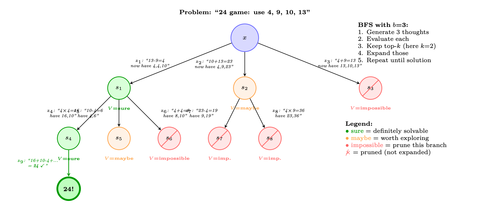
Figure 13.3: Tree-of-Thoughts on the "Game of 24" task: use operations on 4, 9, 10, 13 to make 24. At each level, the model generates b = 3 candidate thoughts, evaluates each (sure/maybe/impossible), prunes unpromising branches, and expands the most promising ones. The green path leads to a solution; red paths are pruned early.

5. Repeat until a solution is found or depth limit reached

DFS (Depth-First Search):

1. Generate b candidate thoughts for current state

2. Evaluate: if V (s) = impossible, backtrack immediately

3. If V (s) = sure/maybe, recurse deeper (pick the most promising)

4. If depth limit reached without solution, backtrack

5. Continue until solution found or all branches explored

ToT: Value Evaluation Prompt

# The LLM evaluates partial reasoning states: EVAL_PROMPT = """Evaluate if this partial solution can reach 24.

Numbers remaining: [4, 4, 10] Steps so far: 13 - 9 = 4

Can these remaining numbers (4, 4, 10) be combined using +,-,*,/ to make 24?

Analysis: 4 * (10 - 4) = 4 * 6 = 24. Yes!

Judge: sure/maybe/impossible Answer: sure"""

# Thought generation prompt: GEN_PROMPT = """Input: 4 9 10 13 Possible next steps: 1. 13 - 9 = 4 (left: 4 4 10) 2. 10 + 13 = 23 (left: 4 9 23) 3. 9 - 4 = 5 (left: 5 10 13) ..."""

Computational Cost. For ToT with branching factor b, depth d, and beam width k:

LLM calls (BFS) = k · b |{z} generation + k · b |{z} evaluation = 2kb per level =⇒Total = 2kbd (13.6)

13.2.4 Graph-of-Thoughts (GoT)

Graph-of-Thoughts [235] extends ToT from a tree to a directed acyclic graph (DAG), introducing a critical capability: merging partial solutions from different branches. This allows the model to synthesize insights from multiple reasoning paths into a single refined solution.

Key Operations. GoT introduces three operations beyond ToT:

• Generate: Produce new thoughts from a state (same as ToT)

• Aggregate/Merge: Combine multiple thoughts into one refined thought -- this is impossible in a tree

• Refine: Iteratively improve a thought based on feedback

• Score: Evaluate thought quality (same as ToT's value function)

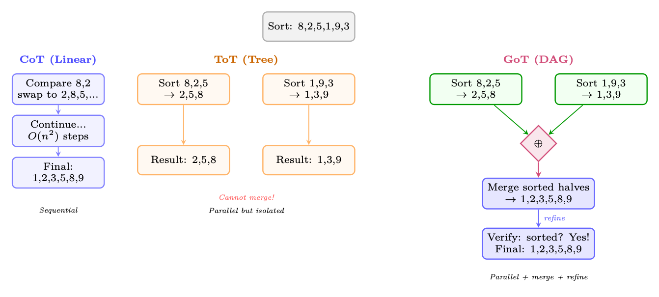
Figure 13.4: Comparison of CoT (linear chain), ToT (tree -- branches but no merging), and GoT (DAG -- branches can merge). For a sorting task, GoT can split the array into sub-problems, solve them independently (parallel), then merge the results -- impossible in a pure tree structure. This enables divide-and-conquer reasoning.

Graph Operations (formal). Let V = {v1, . . . , vn} be thought vertices and E ⊆V ×V be directed edges. GoT supports:

Generate(v) : v →{vc1, . . . , vcb} (create children) (13.7)

Aggregate(v1, . . . , vk) →vmerged (merge k thoughts into one) (13.8)

Refine(v, n) →v′ (improve v through n iterations) (13.9)

Score(v) →s ∈[0, 1] (evaluate thought quality) (13.10)

The Aggregate operation is the key differentiator: it creates edges from multiple parent nodes to a single child, forming a DAG rather than a tree. This enables:

• Divide-and-conquer: Split problem →solve sub-problems in parallel →merge solutions

• Ensemble reasoning: Generate multiple perspectives, then synthesize the best ideas

13.2.5 Best-of-N with Reward Models

Best-of-N (BoN) [196, 236] is the simplest scaling method that uses a learned reward model to select among candidates:

y∗= arg max y∈{y1,...,yN} Rϕ(x, y), yi ∼πθ(·|x) (13.11)

Variants by reward model type:

• BoN with ORM: Score complete solutions; select the highest-scoring one. Equivalent to Self-Consistency when ORM ≈correctness check.

• BoN with PRM: Score at each reasoning step; select the solution with highest minimum step score (least likely to have an error at any step).

• Weighted BoN: Weight candidates by reward: y∗∼softmax(R(y1)/τ, . . . , R(yN)/τ).

BoN Scaling Law

For a model with per-sample accuracy p, the probability of at least one correct sample in N tries:

P(success with BoN) = 1 −(1 −p)N (13.12)

With a perfect reward model (oracle that always selects correctly):

• p = 0.3, N = 10: success = 97%

• p = 0.1, N = 50: success = 99.5%

In practice, imperfect reward models cap the effective N -- beyond N ≈64-256, reward model errors dominate and accuracy plateaus or decreases (reward hacking).

13.2.6 Monte Carlo Tree Search (MCTS) for Reasoning

MCTS [19, 237] combines the structured exploration of ToT with learned value estimates and visit-count statistics to allocate inference compute optimally. Originally developed for game-playing (AlphaGo [19]), MCTS has been adapted for LLM reasoning by systems including AlphaProof [238] and rStar [239].

Algorithm (adapted for LLM reasoning). Each MCTS iteration consists of four phases:

UCB for Reasoning. Node selection uses PUCT (Predictor + UCB applied to Trees):

"

#

pP b N(s, b) 1 + N(s, a)

a∗= arg max a

Q(s, a) + cpuct · P(s, a) ·

(13.13)

where P(s, a) = πθ(a|s) is the LLM's prior probability of generating step a from state s. This biases exploration toward steps the LLM already considers likely, while the UCB term encourages trying under-explored alternatives.

MCTS for Math Reasoning: Running Example

Problem: Prove that √

2 is irrational. Iteration 1 (Selection →root, Expansion):

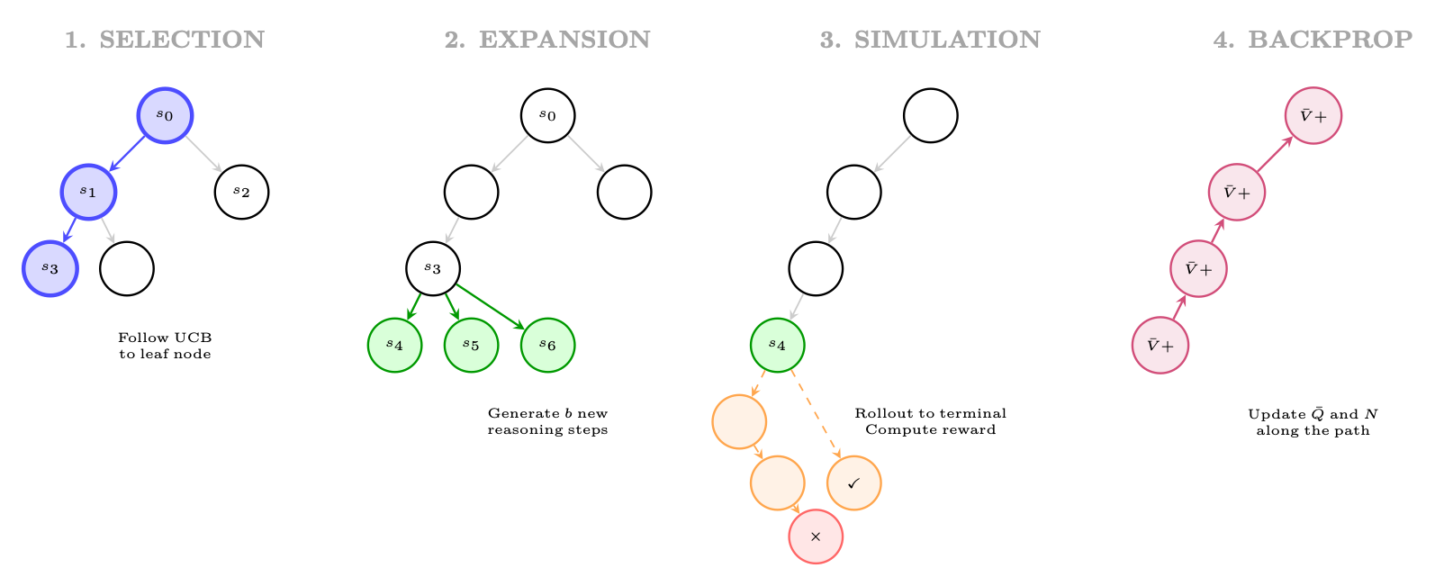
Figure 13.5: Four phases of MCTS for reasoning: (1) Selection: traverse tree using UCB to find a promising leaf; (2) Expansion: generate new reasoning steps from the leaf; (3) Simulation: complete the reasoning to a terminal state and evaluate; (4) Backpropagation: update value estimates along the path.

• Generate 3 candidate first steps:

1. "Assume for contradiction that √

2 = p/q in lowest terms." (P = 0.7)

2. "Consider the decimal expansion of √

2 = 1.414..." (P = 0.15)

3. "Use the fundamental theorem of arithmetic." (P = 0.10)

• Rollout from z1: reaches correct proof in 4 steps →r = 1.0

• Rollout from z2: fails (decimal doesn't prove irrationality) →r = 0.0

• Backprop: Q(s0, z1) = 1.0, N(s0, z1) = 1

Iteration 2 (Selection: pick z1 by UCB):

• Expand from state "Assume √

2 = p/q...":

1. "Then 2 = p2/q2, so p2 = 2q2." (P = 0.8)

2. "Then p and q share no common factors." (P = 0.15)

• Rollout from z4: correct continuation →r = 1.0

• Backprop: Q(s0, z1) = 1.0, Q(s1, z4) = 1.0

After 20 iterations: The tree has explored 8 distinct reasoning paths. The most-visited path is selected as the final proof: z1 →z4 →z6 →z8 (classical proof by contradiction via even/odd argument).

Comparison: ToT vs. MCTS.

13.2.7 Beam Search over Reasoning Steps

Beam search -- long standard in NMT and text generation -- can be applied at the reasoning step level rather than the token level. Instead of tracking the top-k token sequences, we track the top-k reasoning prefixes:

d X

(

)

Bd = top-k

(s1, . . . , sd) :

i=1 log πθ(si|s<i) + λ · Vϕ(s1, . . . , sd)

(13.14)

Dimension ToT MCTS

Value estimation LLM prompt ("sure/maybe/impossible") Learned value network + rollout statistics

Exploration Fixed beam width; no revisiting UCB adaptively allocates budget to promising nodes Compute allocation Uniform across depth levels Focused: more simulations on harder subproblems Training integration No training; pure prompting Can distill MCTS policy into the base model [19] Best for Simple branching problems (24 game) Complex problems requiring deep exploration (proofs, code)

13.2.8 Iterative Refinement and Self-Correction

Rather than exploring breadth (multiple parallel chains), iterative refinement invests compute in depth -- repeatedly improving a single solution:

y(t+1) = LLM � "Improve this solution:", y(t), "Errors found:", e(t)� (13.15)

where e(t) may come from:

• Self-verification: Ask the model to check its own answer

• External verification: Run code, check math symbolically

• Critic model: A separate model identifies errors

Notable methods: Self-Refine [240] (iterative self-feedback), Reflexion [224] (verbal RL via reflections stored in memory), and LATS [225] (tree search + reflection-based pruning).

13.2.9 Method Comparison and Selection Guide

Table 13.2: Comprehensive comparison of test-time scaling methods.

Method Structure LLM Calls Parallelizable Needs RM? Best For

CoT [122] Chain 1 N/A No Easy-medium problems Self-Consistency [124] Parallel chains N ✓Fully No (majority vote) Math with discrete answers Best-of-N + ORM Parallel chains N + 1 ✓Fully Yes (ORM) General tasks with good RM Best-of-N + PRM Parallel chains N + N·K ✓Fully Yes (PRM) Complex multi-step reasoning ToT [234] Tree (BFS/DFS) O(kbd) Partial LLM-as-judge Structured search problems GoT [235] DAG O(kbd) Partial LLM-as-judge Decomposable problems MCTS [237] Tree + values O(Nsim · d) Partial Yes (value net) Hard proofs, coding Self-Refine [240] Linear (iterative) 2T No Self-critic Open-ended generation LATS [225] Tree + reflection O(N · d) Partial LLM-as-judge Agent tasks

When to Use Which Method

• Budget < 5× base cost: Use CoT or Self-Consistency. Maximum bang for the buck.

• Budget 5-50×: Use Best-of-N with PRM (if you have a good reward model) or ToT-BFS with b = 3, k = 2.

• Budget 50-500×: Use MCTS with a trained value function. This is the regime where DeepSeek-R1 and OpenAI o1 operate -- long reasoning chains with implicit tree search.

• Parallelism required: Self-Consistency and Best-of-N are fully parallel; ToT/MCTS require sequential depth expansion.

• No reward model available: Use Self-Consistency (majority vote) or ToT with LLM-asjudge evaluation.

The Implicit Test-Time Scaling in Reasoning Models

Modern reasoning models (DeepSeek-R1 [15], OpenAI o1/o3 [241, 242]) perform implicit testtime scaling via long chain-of-thought generation. Their "thinking" tokens serve a function analogous to MCTS rollouts: the model explores multiple approaches, backtracks ("Wait, let me reconsider..."), verifies intermediate steps, and allocates more tokens to harder sub-problems. The key insight of R1/o1 training is that GRPO/RL teaches the model to perform this implicit search within a single generation, eliminating the need for external orchestration (ToT prompts, MCTS infrastructure). The model becomes its own search algorithm.

13.3 DeepSeek-R1

DeepSeek-R1 [15] is the first fully open-source large reasoning model to match or exceed OpenAI o1 on major benchmarks. Its training pipeline is technically transparent and has become the de facto reference implementation for RL-based reasoning.

13.3.1 Two-Stage Training Pipeline

Stage 1: Cold-Start Supervised Fine-Tuning The base model (DeepSeek-V3) is first fine-tuned on a small, carefully curated dataset of long chain-of-thought examples. This "cold start" phase serves two purposes:

1. Format initialization: The model learns to produce reasoning in the <think>...</think> format before emitting a final answer.

2. Stability: Without cold-start SFT, pure RL from scratch on the base model produces unstable training dynamics and degenerate outputs (e.g., language mixing, repetitive loops).

The cold-start dataset contains only ∼thousands of examples, deliberately kept small to avoid over-constraining the reasoning style that RL will later discover.

Stage 2: GRPO-Based Reinforcement Learning After cold-start SFT, the model undergoes large-scale RL using Group Relative Policy Optimization (GRPO). The full GRPO objective as used in R1 is described in Section 13.3.3.

1. Base model: DeepSeek-V3 (671B MoE, 37B active parameters)

2. Cold-start SFT: ∼thousands of long-CoT examples, format: <think>...</think><answer>...</answer>

3. RL phase: GRPO with verifiable rewards on math + code problems

4. Rejection sampling: Generate multiple solutions, keep correct ones

5. SFT on RL outputs: Fine-tune on high-quality RL-generated chains

6. Final RL: Second RL phase for alignment + helpfulness

13.3.2 Reward Design: Accuracy and Format Rewards

A key design choice in R1 is the absence of a process reward model. Instead, R1 uses two simple, automatically computable rewards:

Accuracy Reward For math problems with verifiable answers:

( 1 if verify(y, y∗) = True 0 otherwise (13.16)

racc(y, y∗) =

where y is the model's final answer (extracted from <answer> tags) and y∗is the ground-truth answer. The verify function uses symbolic math comparison (e.g., SymPy) to handle equivalent forms. For code problems, the accuracy reward is determined by passing test cases:

rcode acc (y, T ) = 1 |T |

X

t∈T 1[execute(y, t) = expected(t)] (13.17)

Format Reward To enforce the <think>...</think> structure:

( 1 y has valid <think> and <answer> tags 0 otherwise (13.18)

rfmt(y) =

Combined Reward r(y, y∗) = racc(y, y∗) + λfmt · rfmt(y) (13.19)

with λfmt = 0.1 in the original implementation (small enough not to dominate, large enough to prevent format collapse).

No Process Reward Model A notable and surprising finding of R1 is that no process reward model (PRM) is needed. Despite the long reasoning chains, outcome-only rewards are sufficient for RL to discover highquality reasoning strategies. The authors hypothesize that the verifiable nature of math/code rewards provides sufficient signal, and that PRMs introduce their own failure modes (reward hacking at the step level). This contrasts with the approach taken by OpenAI (Section 13.4).

13.3.3 GRPO Formulation for R1

{yi}G i=1 ∼πθ(· | q) (13.20)

Compute rewards {ri}G i=1 using the reward function from Eq. [eq:r1_combined_reward]. The normalized advantage for response i is:

ˆAi = ri −µr

σr + ϵ (13.21)

G PG i=1 ri, σr = q

1 G PG i=1(ri −µr)2, and ϵ = 10−8 for numerical stability.

where µr = 1

GRPO Objective The GRPO objective clips the probability ratio (as in PPO) and adds a KL penalty against a reference policy πref:

|yi| X

G X

" 1 G

1 |yi|

LGRPO(θ) = −Eq∼D, {yi}∼πθ(·|q)

i=1

t=1

#

min � ρi,t ˆAi, clip(ρi,t, 1−ε, 1+ε) ˆAi � −β DKL[πθ ∥πref]

(13.22)

where:

• ρi,t = πθ(yi,t | q, yi,<t) πθold(yi,t | q, yi,<t) is the per-token probability ratio

• ε ∈{0.1, 0.2} is the PPO clipping parameter

• β > 0 controls the KL penalty strength

• |yi| is the length of response i (length normalization prevents bias toward short responses)

KL Penalty Formulation The KL divergence term is computed token-by-token:





 |y| X

t=1 log πθ(yt | q, y<t)

DKL[πθ ∥πref] = Ey∼πθ(·|q)

 (13.23)

πref(yt | q, y<t)

In practice, R1 uses an unbiased estimator of the KL that avoids computing πref at every step by using the approximation:

DKL[πθ ∥πref] ≈πref(yt | q, y<t)

πθ(yt | q, y<t) −log πref(yt | q, y<t)

πθ(yt | q, y<t) −1 (13.24)

which is always non-negative and equals zero when πθ = πref.

GRPO in Practice: Group Size and Stability

In R1's training, G = 8 responses are sampled per question. This is a critical hyperparameter:

• Too small (G = 2): High variance in advantage estimates; training is noisy.

• Too large (G = 32): Computational cost scales linearly; diminishing returns.

• G = 8: Empirically found to balance variance reduction and compute cost.

The group sampling also provides a natural curriculum signal: as training progresses, the model's average reward µr increases, and the variance σr decreases. Problems where all G responses are correct (or all wrong) contribute zero gradient, naturally focusing learning on problems at the frontier of the model's capability.

A major practical contribution of R1 is demonstrating that reasoning capabilities can be distilled into much smaller models via supervised fine-tuning on R1-generated chains. The R1-Distill series (1.5B, 7B, 8B, 14B, 32B, 70B parameters) is trained by:

1. Generating long-CoT solutions to a large problem set using R1 (671B)

2. Filtering to keep only correct solutions

3. Fine-tuning smaller base models (Qwen2.5, Llama-3) on these solutions

Distillation vs. RL for Small Models A striking finding: distillation outperforms RL training from scratch on small models. DeepSeek-R1-Distill-Qwen-7B achieves higher MATH benchmark scores than a 7B model trained with GRPO directly. This suggests that:

• Small models lack the capacity to discover reasoning strategies via RL exploration

• But they can learn to imitate reasoning strategies discovered by larger models

• The bottleneck for small models is exploration, not representation

The distillation approach raises an important question about the nature of reasoning: is the small model truly "reasoning," or is it pattern-matching on the surface form of reasoning chains? Empirically, distilled models show some generalization to novel problem types, suggesting genuine internalization of reasoning strategies rather than pure memorization.

13.4 OpenAI o1/o3 Series

OpenAI's o1 [241] (released September 2024) and subsequent o3/o4-mini [242] models represent the commercial frontier of reasoning model development. While full technical details remain proprietary, the published system cards, technical reports, and empirical observations provide substantial insight into the methodology.

13.4.1 Chain-of-Thought RL with Hidden Reasoning Tokens

The defining architectural choice of o1 is the use of hidden reasoning tokens: the model generates an internal chain-of-thought (called a "reasoning trace" or "thinking tokens") that is not shown to the user. Only the final answer is returned. This design has several implications:

• No format constraints: The hidden reasoning can use any format, including scratchpad notation, pseudocode, or even non-English reasoning.

• No reward hacking on style: Since users never see the reasoning, there is no pressure to make it look "good" rather than be useful.

• Proprietary protection: The reasoning process is not exposed, preventing direct imitation.

The training procedure is described as "training models to reason using RL," with the RL objective applied to the complete (hidden reasoning + final answer) sequence, rewarded only on the quality of the final answer.

13.4.2 Process Reward Models vs. Outcome Reward Models

RORM(q, y) ∈[0, 1] (13.25)

For verifiable tasks (math, code), this reduces to exact-match verification. For open-ended tasks, a learned reward model is used.

Process Reward Model (PRM) A PRM assigns a reward to each reasoning step sk in the chain y = (s1, s2, . . . , sK):

K X

k=1 γK−k · rk(q, s1, . . . , sk) (13.26)

RPRM(q, y) =

where rk ∈[0, 1] is the step-level reward and γ ∈(0, 1] is a discount factor. The step-level reward rk estimates the probability that the partial solution (s1, . . . , sk) leads to a correct final answer:

rk(q, s1, . . . , sk) = P(correct final answer | q, s1, . . . , sk) (13.27)

PRM vs. ORM: The Credit Assignment Tradeoff

ORM provides clean, unambiguous rewards but suffers from severe credit assignment problems: a single wrong step early in a 50-step chain receives the same zero reward as a completely random response. PRM provides dense rewards that directly address credit assignment, but introduces new challenges:

• Training data: Step-level labels require human annotation or automated generation (MathShepherd, Section 13.6.2).

• Reward hacking: Models can learn to produce steps that look correct to the PRM without actually being correct.

• Distribution shift: PRMs trained on one distribution of reasoning chains may not generalize to the novel chains produced by RL.

The empirical evidence suggests PRMs are beneficial for search (selecting among candidate solutions) but their benefit for training is less clear.

13.4.3 Inference-Time Compute Scaling

The o1 technical report demonstrates a clear scaling law: more thinking tokens monotonically improve performance on hard reasoning tasks. This is operationalized through a "thinking budget" parameter that controls the maximum number of hidden reasoning tokens. Let T be the thinking token budget. The empirical scaling law observed is approximately:

Pass@1(T) ≈a −b · T −c (13.28)

for constants a, b, c > 0, where a represents the asymptotic accuracy ceiling and c characterizes the rate of improvement. For AIME 2024, o1 with full thinking budget achieves ∼83% accuracy, compared to ∼13% for GPT-4o (which uses no extended thinking).

13.4.4 Training Compute vs. Test-Time Compute

A fundamental insight from the o1/o3 series is the compute equivalence principle: there exists a tradeoff curve between training compute Ctrain and test-time compute Ctest such that points on the curve achieve similar performance:

Performance(Ctrain, Ctest) = g(αCp train + βCq test) (13.29)

While o3 and o4-mini details remain largely proprietary, several observations have emerged:

• o3: Substantially larger thinking budgets than o1; achieves near-human performance on ARCAGI (87.5% with high compute). Believed to use more sophisticated search strategies during inference.

• o4-mini: Demonstrates that smaller models with RL-trained reasoning can be highly competitive. Achieves 93% on AIME 2025 with extended thinking, suggesting that model size is less important than reasoning capability for math.

• Tool use: o3/o4-mini integrate tool use (code execution, web search) into the reasoning process, allowing the model to verify intermediate steps programmatically.

13.5 QwQ and Qwen Reasoning Models

Alibaba's Qwen team has developed a series of reasoning models (QwQ-32B [244], Qwen3 [245]) that represent the open-source frontier alongside DeepSeek-R1. Their approach differs in several key respects.

13.5.1 Multi-Stage RL Pipeline

The Qwen reasoning pipeline uses a more elaborate multi-stage approach:

1. Base pretraining: Qwen2.5 base model with strong mathematical and coding capabilities

2. SFT on diverse reasoning: Fine-tuning on a broad mixture of reasoning tasks (math, code, science, logic)

3. Rejection sampling fine-tuning (RFT): Generate N solutions per problem, keep correct ones, fine-tune

4. RL phase 1: GRPO on math and code with verifiable rewards

5. RL phase 2: Broader RL including instruction following and safety

13.5.2 Rejection Sampling + RL Combination

A key innovation in the Qwen approach is the iterative combination of rejection sampling and RL:

1. Initialize: Policy π0 from SFT model.

2. Rejection Sampling: Sample N solutions: {yi}N i=1 ∼πk−1(· | q). Keep correct solutions: Y+(q) = {yi : r(yi, y∗) = 1}.

3. SFT update: πSFT k ←SFT(πk−1, S q Y+(q))

4. RL update: πk ←GRPO(πSFT k , D)

5. Repeat steps 2-4 for K iterations to obtain final policy πK.

QwQ-32B and Qwen3 models support tool-integrated reasoning: the model can invoke external tools (Python interpreter, search engine, calculator) during its reasoning chain. This is implemented via special tokens:

<think > Let me solve this step by step. First , I'll compute the eigenvalues of the matrix.

<tool_call > {" name ": "python", "arguments ": {" code ": "import numpy as np\nA = np.array ([[2 ,1] ,[1 ,3]])\neigenvalues = np.linalg.eigvals(A)\nprint(eigenvalues)"}} </tool_call >

<tool_response > [1.38196601 3.61803399] </tool_response >

The eigenvalues are approximately 1.382 and 3.618. These are (5 +/- sqrt5)/2, which are the golden ratio and its conjugate ... </think > <answer >The eigenvalues are (5 +/- sqrt5)/2</answer >

Listing 13.1: Tool-integrated reasoning format in QwQ

The RL training reward is computed on the final answer, but the model learns to use tools strategically because tool use improves the probability of reaching the correct answer.

13.6 Key Methods with Mathematical Foundations

13.6.1 Monte Carlo Tree Search for Reasoning

Monte Carlo Tree Search (MCTS) provides a principled framework for reasoning as tree search. In the AlphaProof [238] and related systems, MCTS is applied over reasoning steps rather than game moves.

State and Action Space

• State sk: The partial reasoning chain (q, r1, r2, . . . , rk) where ri are reasoning steps

• Action a: The next reasoning step (a sentence or paragraph)

• Terminal state: A state containing a final answer

• Reward: R(sterminal) = racc (Eq. [eq:r1_accuracy_reward])

Value Function for Partial Solutions A value function V (sk) estimates the probability of reaching a correct answer from partial state sk:

M X

V (sk) = P(correct answer | sk) ≈1

m=1 R(rolloutm(sk)) (13.30)

M

where rolloutm(sk) is a Monte Carlo rollout from sk to a terminal state using the current policy.

UCB Exploration Node selection uses the Upper Confidence Bound (UCB) formula adapted for reasoning:

p

N(sk) 1 + N(sk, a) (13.31)

UCB(sk, a) = Q(sk, a) + cpuct · πθ(a | sk) ·

• πθ(a | sk) is the policy prior (language model probability of step a)

• N(sk) is the visit count of state sk

• N(sk, a) is the visit count of the (sk, a) edge

• cpuct is the exploration constant

MCTS-Guided Training MCTS can be used to generate high-quality training data:

LMCTS(θ) = − X

X

a πMCTS(a | sk) log πθ(a | sk) (13.32)

k

where πMCTS(a | sk) ∝N(sk, a)1/τ is the MCTS policy (visit count distribution with temperature τ).

13.6.2 Process Reward Models

Math-Shepherd: Automated PRM Training Math-Shepherd [246] proposes an automated method for training PRMs without human step-level annotations. The key insight is to use outcomebased estimation: a step sk is labeled as correct if there exists a completion from sk that reaches the correct answer. Formally, for a partial solution (s1, . . . , sk):

ˆrk = 1[∃(sk+1, . . . , sK) : verify(sK, y∗) = 1] (13.33)

In practice, this is estimated by sampling M completions from sk and checking if any are correct:

" M X

#

m=1 verify(completem(sk), y∗) > 0

ˆrk ≈1

(13.34)

The PRM is then trained with binary cross-entropy:

K X

LPRM(ϕ) = −

k=1 [ˆrk log rϕ(sk) + (1 −ˆrk) log(1 −rϕ(sk))] (13.35)

PRM for Best-of-N Selection A primary application of PRMs is best-of-N selection: generate N candidate solutions and select the one with the highest PRM score:

y∗= arg max y∈{y1,...,yN} RPRM(q, y) (13.36)

This is more effective than majority voting (which uses ORM) because PRM can distinguish between solutions that reach the same answer via different quality reasoning paths.

13.6.3 Outcome Reward Models and Majority Voting

Majority Voting (Self-Consistency) The simplest form of test-time compute scaling is majority voting [124]: generate N solutions and return the most common answer:

N X

y∗= arg max a

i=1 1[yi = a] (13.37)

Under the assumption that each solution is independently correct with probability p > 0.5, the probability that majority voting is correct is:

N X

!

pk(1 −p)N−k N→∞ −−−−→1 (13.38)

P(majority correct) =

N X

y∗= arg max a

i=1 RORM(q, yi) · 1[yi = a] (13.39)

13.6.4 Self-Play for Reasoning

Self-play methods generate training data by having the model play both the generator and verifier roles.

STaR: Self-Taught Reasoner STaR [223] bootstraps reasoning capabilities iteratively:

1. Generate reasoning chains for a problem set

2. Keep chains that lead to correct answers (rejection sampling)

3. Fine-tune on kept chains

4. Repeat with the improved model

The key insight is that the model can rationalize correct answers: even if it cannot solve a problem from scratch, it can generate a plausible reasoning chain given the answer, which can then be used as training data.

Self-Play RL In self-play RL for reasoning, the model generates both problems and solutions:

Lself-play(θ) = Eq∼πgen θ Ey∼πsolve θ (·|q) [r(y, y∗)] (13.40)

where πgen θ generates problems and πsolve θ solves them. The generator is rewarded for producing problems that are challenging but solvable.

13.6.5 Reinforcement Learning from Verifiable Rewards (RLVR)

RLVR [247] is a framework that uses ground-truth verification as the reward signal, applicable to any domain where correctness can be automatically checked.

Verifiable Domains

• Mathematics: Symbolic verification via SymPy, Lean, or Isabelle

• Code: Unit test execution

• Formal logic: Proof checking

• Factual QA: Database lookup

• Games: Win/loss outcome

RLVR Objective

LRLVR(θ) = −E(q,y∗)∼DEy∼πθ(·|q) [verify(y, y∗)] + βDKL[πθ ∥πref] (13.41)

In code generation, the verifier is a test suite. A model trained with RLVR can learn to:

• Hardcode test outputs: Return the expected output for each test input without implementing the actual algorithm

• Exploit weak tests: Pass all provided tests while failing on edge cases

Mitigations include: using large, diverse test suites; including adversarial test cases; using executionbased rewards that penalize hardcoding (e.g., checking that the solution runs in O(n log n) time).

13.6.6 Journey Learning

Journey Learning [248] proposes training on the full reasoning trajectory, including failed attempts and corrections, rather than only successful final solutions.

Motivation Standard rejection sampling discards failed attempts. But failed attempts contain valuable information:

• Which approaches don't work (negative examples)

• How to recognize and recover from errors (correction patterns)

• The structure of the problem space (exploration data)

Journey Learning Objective Given a trajectory τ = (s0, a0, s1, a1, . . . , sT ) that may include backtracking:

T X

Ljourney(θ) = −

t=0 wt log πθ(at | st) (13.42)

where the weights wt are designed to emphasize:

• Steps that lead to eventual success (wt > 1)

• Correction steps after errors (wt > 1)

• Steps in failed branches (wt < 1, but > 0)

13.6.7 Quiet-STaR: Reasoning at Every Token

Quiet-STaR [230] extends the reasoning paradigm to every token position: rather than generating a reasoning chain only before the final answer, the model generates a "thought" at every token position.

Formulation For each token position t, the model generates a hidden thought zt before predicting the next token xt+1: P(xt+1 | x≤t) = Ezt∼πθ(·|x≤t) [πθ(xt+1 | x≤t, zt)] (13.43)

In practice, this is approximated by mixing the predictions with and without the thought:

P(xt+1 | x≤t) = α · πθ(xt+1 | x≤t, zt) + (1 −α) · πθ(xt+1 | x≤t) (13.44)

Training with REINFORCE Since the thought zt is a discrete latent variable, the gradient is estimated using REINFORCE:

∇θLQS = Ezt [∇θ log πθ(zt | x≤t) · (log P(xt+1 | x≤t, zt) −bt)] (13.45)

Quiet-STaR increases inference cost by a factor of Lz + 1 where Lz is the thought length, applied at every token position. For a sequence of length T with thoughts of length Lz = 8, this is a 9× increase in compute. This makes Quiet-STaR impractical for long sequences without significant engineering optimizations (e.g., speculative decoding for thoughts, caching).

13.7 Scaling Laws for Reasoning

Recent work [249, 250] has established that test-time compute scales predictably with reasoning performance, extending the classical scaling laws [251] into the inference regime.

13.7.1 Training Compute vs. Test-Time Compute Tradeoff

The fundamental scaling question for reasoning models is: given a fixed total compute budget Ctotal = Ctrain + N · Ctest (where N is the number of queries), how should compute be allocated? Let A(Ctrain, Ctest) denote the accuracy of a model trained with Ctrain FLOPs and given Ctest inference FLOPs per query. Empirically:

A(Ctrain, Ctest) ≈1 −exp � −a · Cα train · Cβ test � (13.46)

for constants a, α, β > 0. The optimal allocation for a fixed total budget Ctotal satisfies the condition that marginal return per FLOP is equalized between training and inference:

∂A ∂Ctrain = 1

N · ∂A ∂Ctest (13.47)

Intuitively: one FLOP of training benefits all N queries, while one FLOP of test-time benefits only one query. At the optimum, the per-query marginal value of test-time compute is N times larger than training compute (because training is amortized). Applying this to Eq. [eq:reasoning_scaling_law] gives the optimal training compute fraction:

C∗ train Ctotal = α α + β (13.48)

For the specific budget structure Ctotal = Ctrain + N · Ctest, this fraction is independent of N under the multiplicative accuracy model. However, in practice α and β are problem-dependent: for high-volume deployments (large N), even small improvements in the base model dominate, favoring training investment. For low-volume, high-stakes queries (small N), test-time compute is more cost-effective.

13.7.2 When to Invest in Longer Chains vs. Better Base Models

Reasoning Chain Length vs. Model Capacity

The optimal reasoning chain length L∗for a model of capacity C on a problem of difficulty D satisfies: L∗∝D

Cγ (13.49)

for some γ > 0. This implies:

• Hard problems require longer chains regardless of model size

• Larger models require shorter chains for the same problem difficulty

• Diminishing returns: Beyond L∗, additional tokens provide no benefit and may hurt (overthinking)

• Accumulation of errors in long chains (error propagation)

• Distraction from the main solution path

• Overconfidence in incorrect intermediate conclusions

13.7.3 Optimal Token Budget Allocation

For a model with a fixed token budget B, the allocation between "thinking" tokens Tthink and "answering" tokens Tanswer should satisfy:

T ∗ think = arg max T A(T, B −T) (13.50)

Empirically, the optimal split is problem-dependent:

• Simple problems: T ∗ think/B ≈0.3 (30% thinking)

• Hard problems: T ∗ think/B ≈0.8 (80% thinking)

• Very hard problems: T ∗ think/B ≈0.95 (95% thinking, minimal answer)

This motivates adaptive thinking budgets: allocating more tokens to harder problems, which can be estimated by the model's uncertainty on initial solution attempts.

13.8 Comparison of Reasoning Models

Table 13.3: Comparison of training methodologies for reasoning models.

Method PRM ORM MCTS Distill Tool Open

OpenAI o1/o3 ✓ ✓ Unknown ✓ × DeepSeek-R1 × ✓ × ✓ × ✓ QwQ / Qwen3 Partial ✓ × × ✓ ✓ AlphaProof ✓ ✓ ✓ ✓ × Math-Shepherd ✓ ✓ × × ✓ STaR / Quiet-STaR × ✓ × × ✓

13.9 Summary and Open Problems

The field of RL for reasoning models has advanced remarkably rapidly. Several key lessons have emerged:

1. Verifiable rewards are sufficient: For domains with ground-truth verification (math, code), outcome-only rewards are sufficient for RL to discover sophisticated reasoning strategies, without requiring process reward models.

2. Test-time compute is a new axis: Reasoning models introduce a new dimension of scaling-- inference compute--that is roughly substitutable with training compute for hard reasoning tasks.

3. Distillation is highly effective: Large reasoning models can transfer their capabilities to much smaller models via supervised fine-tuning on generated chains, often outperforming direct RL training of small models.

4. Emergent meta-cognition: RL training on reasoning tasks produces emergent self-correction and verification behaviors that were not explicitly trained.

Several fundamental questions remain open:

• Generalization: Do reasoning capabilities trained on math/code transfer to other domains (scientific reasoning, planning, social reasoning)?

• Faithfulness: Are the generated reasoning chains causally responsible for the final answer, or are they post-hoc rationalizations?

• Optimal search: What is the optimal search strategy during inference--beam search, MCTS, or something else?

• Reward design: For domains without ground-truth verifiers, how can we design reliable reward signals for reasoning?

• Overthinking: How can models learn to allocate the right amount of thinking--neither too little nor too much?

• Compositional reasoning: Can RL-trained reasoning models solve problems that require composing multiple distinct reasoning skills?

The development of reasoning models represents a paradigm shift: from language models that know things to language models that can figure things out. The RL methods described in this section are the primary engine driving this shift, and their continued development is likely to be a central focus of AI research in the coming years.

Part IV

Evaluation