Preference Optimization Variants

Preference Optimization Variants

This chapter covers the family of methods that extend or replace DPO with different objectives, data assumptions, or architectural trade-offs. Each addresses a specific limitation of standard offline DPO: distribution shift (Online DPO), the need for paired data (KTO), overfitting to noisy labels (IPO), reference model memory cost (ORPO), or training complexity (Best-of-N).

8.1 Online DPO

8.1.1 Motivation

Standard DPO's primary limitation: the preference data was generated by a different model (often an older checkpoint or even a different model family). As training progresses, the policy generates text that looks nothing like the training pairs →the loss is optimizing on an irrelevant distribution. Online DPO solution [195]: Generate fresh preference pairs from the current policy at every step, judge them with a reward model, then apply the DPO loss.

8.1.2 Algorithm

1. Generate K responses per prompt from current πθ

2. Score all responses with reward model rϕ

3. Create pairs: highest-scoring = chosen, lowest-scoring = rejected

4. Apply DPO loss on these fresh pairs

5. Repeat (new generation every step)

Online DPO = Best of Both Worlds

• From DPO: simple supervised loss, no value function, no GAE, stable optimization

• From PPO: on-policy data, self-improvement beyond dataset, no distribution shift

• Key difference from GRPO: uses DPO loss (pair-based) instead of PPO loss (per-sample advantage)

Trade-off: Needs a reward model (DPO doesn't), but no value head (PPO does). Middle ground complexity.

8.1.3 TRL Implementation

from trl import OnlineDPOConfig , OnlineDPOTrainer from transformers import AutoModelForCausalLM , AutoModelForSequenceClassification

model = AutoModelForCausalLM . from_pretrained ("meta -llama/Llama -3.1 -8B-Instruct",

torch_dtype=torch.bfloat16) reward_model = AutoModelForSequenceClassification . from_pretrained (

"RLHFlow/ArmoRM -Llama3 -8B-v0.1", torch_dtype=torch.bfloat16)

online_dpo_config = OnlineDPOConfig (

output_dir="./ online_dpo_output ", learning_rate =5e-7, beta =0.1, # DPO beta (same meaning as standard DPO) num_generations =4, # K responses per prompt per_device_train_batch_size =4, gradient_accumulation_steps =4, max_new_tokens =512, temperature =0.7, bf16=True , num_train_epochs =1, logging_steps =10, )

trainer = OnlineDPOTrainer (

model=model , reward_model=reward_model , args=online_dpo_config , train_dataset=prompt_dataset , tokenizer=tokenizer , ) trainer.train ()

8.1.4 Online DPO vs Offline DPO vs PPO

Data Models Loss Best For

Offline DPO Static pairs 2 (policy + reference) DPO Quick alignment, limited compute Online DPO Fresh from πθ 3 (policy + reference + reward model) DPO When DPO plateaus, need exploration PPO Fresh from πθ 4 (policy + reference + reward model + value head) PPO clip Max quality, complex reasoning

8.2 KTO -- Kahneman-Tversky Optimization

8.2.1 Motivation

DPO requires paired preferences: for the same prompt, you need both a good and bad response. In practice, most feedback is unpaired: users give thumbs up/down on individual responses, with no matched pair. KTO's insight [11]: Use prospect theory (from behavioral economics). Humans feel losses more strongly than gains. A "thumbs down" should produce a stronger gradient than a "thumbs up."

8.2.2 Loss Function

LKTO = Eyw [λw(1 −v(x, yw))] + Eyl [λl · v(x, yl)] (8.1)

where v(x, y) = σ � β log πθ(y|x)

Desirable responses (yw): The model gets "utility" from increasing their probability. But with diminishing returns -- once it's already quite likely, don't push harder. Undesirable responses (yl): Loss aversion means the penalty for generating bad text is weighted more strongly than the reward for good text. Default: λl = 1.0, λw = 1.0, but you can set λl > λw. Key advantage: Each training example is independent! No need to find matched pairs. Can use thumbs-up/down data directly.

KTO Data Format Unlike DPO which needs: {"prompt": ..., "chosen": ..., "rejected": ...} KTO only needs: {"prompt": ..., "completion": ..., "label": true/false} This means you can use:

• Thumbs up/down from production traffic

• Upvotes/downvotes from forums

• Human ratings binarized (4-5 stars = good, 1-2 = bad)

• Any per-response quality signal

8.2.3 TRL Implementation

The following shows a minimal working example using HuggingFace TRL.

from trl import KTOConfig , KTOTrainer

# Dataset format: {" prompt ": str , "completion ": str , "label ": bool} # label=True for desirable , label=False for undesirable kto_dataset = [

{"prompt": "What 's 2+2?", "completion": "The answer is 4.", "label": True}, {"prompt": "What 's 2+2?", "completion": "It might be 5.", "label": False}, ]

kto_config = KTOConfig(

output_dir="./ kto_output", beta =0.1, desirable_weight =1.0, # Weight for good examples undesirable_weight =1.0, # Weight for bad examples (increase for loss aversion)

learning_rate =5e-7, max_length =2048 , per_device_train_batch_size =4, gradient_accumulation_steps =4, num_train_epochs =1, bf16=True , )

trainer = KTOTrainer(

model=model , ref_model=ref_model , # Or None with LoRA args=kto_config , train_dataset=kto_dataset , tokenizer=tokenizer , ) trainer.train ()

8.2.4 When to Choose KTO

• One class dominates (e.g., 90% good, 10% bad) -- KTO handles imbalance better

• Rapid iteration with noisy labels (more robust than DPO to noise)

8.3 IPO -- Identity Preference Optimization

8.3.1 Motivation

DPO has a degenerate solution: it can achieve zero loss by making the margin between chosen and rejected infinitely large. In practice, this means DPO overfits -- pushing chosen probability to 1 and rejected to 0, memorizing training data. IPO's fix [12]: Instead of log-sigmoid (which saturates), use a squared loss that targets a specific margin. The loss is minimized at a finite gap, not at infinity.

8.3.2 Loss Function

�2#

"� log πθ(yw|x)

πref(yw|x) −log πθ(yl|x)

πref(yl|x) −1

LIPO = E

(8.2)

2β

IPO vs DPO: Regularization Through Target Margin

DPO: σ(margin) →1 optimally. Margin →∞. No natural stopping point. IPO: Margin → 1 2β optimally. Squared loss penalizes both too-small and too-large margins. Result: IPO is more robust to noisy labels (a mislabeled pair gets bounded influence), and generalizes better because it doesn't memorize.

8.3.3 TRL Implementation

The following shows a minimal working example using HuggingFace TRL.

from trl import DPOConfig , DPOTrainer

# IPO is implemented as a DPO loss_type variant in TRL ipo_config = DPOConfig(

output_dir="./ ipo_output", beta =0.1, loss_type="ipo", # The key difference! learning_rate =5e-7, max_length =2048 , per_device_train_batch_size =4, gradient_accumulation_steps =8, bf16=True , num_train_epochs =1, )

trainer = DPOTrainer(

model=model , ref_model=None , args=ipo_config , train_dataset=pref_dataset , tokenizer=tokenizer , peft_config=lora_config , ) trainer.train ()

8.3.4 When to Choose IPO over DPO

• Noisy preference data (crowdsourced, AI-judged with errors)

• Observing DPO overfitting (train loss →0 but eval degrades)

8.4 ORPO -- Odds Ratio Preference Optimization

8.4.1 Motivation

All methods so far need a reference model -- either as a separate copy (doubles memory) or implicitly via LoRA. ORPO [13] eliminates the reference entirely by combining SFT and preference alignment in a single loss. Key insight: Use the odds ratio of generating chosen vs rejected as the preference signal. The SFT component naturally prevents collapse (no need for KL regularization).

8.4.2 Loss Function

−λ · log σ � log oddsθ(yw|x)

�

LORPO = LSFT(yw) | {z } standard NLL on chosen

(8.3)

oddsθ(yl|x)

| {z } preference alignment via odds ratio

where oddsθ(y|x) = Pθ(y|x) 1−Pθ(y|x).

ORPO: SFT + Alignment in One Shot

SFT term: Trains the model to generate the chosen response well (standard language modeling). Odds ratio term: Additionally pushes the model to prefer chosen over rejected. The odds ratio is a natural contrast that doesn't require a reference model. Why no reference needed?: The SFT loss already anchors the model to reasonable text. It serves the same role as KL-to-reference in other methods. One model, one forward pass, one loss. 50% less memory!

8.4.3 TRL Implementation

The following shows a minimal working example using HuggingFace TRL.

from trl import ORPOConfig , ORPOTrainer

orpo_config = ORPOConfig(

output_dir="./ orpo_output", beta =0.1, # Odds ratio weight (lambda) learning_rate =5e-7, max_length =2048 , per_device_train_batch_size =2, gradient_accumulation_steps =8, bf16=True , num_train_epochs =1, gradient_checkpointing =True , )

trainer = ORPOTrainer(

model=model , # No ref_model needed! args=orpo_config , train_dataset=pref_dataset , # Same format as DPO: prompt/chosen/rejected tokenizer=tokenizer , peft_config=lora_config , ) trainer.train ()

8.4.4 When to Choose ORPO

• Want simplest possible pipeline: one model, one loss, one training run

• Good preference data available from the start

ORPO Limitations

• Less studied than DPO/PPO -- fewer proven recipes at 70B+ scale

• The SFT component means it needs high-quality chosen responses (not just relative preference)

• Harder to debug: two loss components can conflict

See Also: SimPO SimPO [183] is another reference-free preference method that uses length-normalized logprobability as an implicit reward, eliminating the reference model entirely. It is covered in Section 6.9.8 alongside other DPO extensions due to its shared reference-free philosophy.

8.5 Best-of-N Sampling (Rejection Sampling)

8.5.1 Motivation

Sometimes the simplest approach wins. Best-of-N [196] requires no training at all during the RL phase -- just generate multiple candidates and pick the best one.

8.5.2 Algorithm

1. For each prompt, generate N responses from the policy (typically N = 4-64)

2. Score all responses with a reward model

3. Select the highest-scoring response

4. (Optional) Use selected responses as SFT data for the next iteration

Best-of-N response : y∗= arg max yi∼πθ(·|x) rϕ(x, yi) (8.4)

Why Best-of-N is a Legitimate "RL" Method

At inference time: Best-of-N improves output quality without changing model weights. With N = 64, win-rate improves 10-20% over greedy -- sometimes matching or exceeding PPO. As a training method (Rejection Sampling Fine-Tuning / RFT):

1. Generate many responses, select best ones

2. SFT on the selected responses

3. Repeat (iterative refinement)

The following shows a minimal working example using HuggingFace TRL.

from transformers import pipeline import numpy as np

# Inference -time Best -of -N (manual implementation ) gen_pipeline = pipeline("text -generation", model=model , tokenizer=tokenizer)

def best_of_n(prompt , n=16, temperature =0.8): """Generate N candidates and return the highest -reward one.""" candidates = gen_pipeline(

prompt , num_return_sequences =n, temperature=temperature , do_sample=True , max_new_tokens =512 , ) scores = [reward_model.score(prompt , c[" generated_text "]) for c in candidates] return candidates[np.argmax(scores)][" generated_text "]

best_response = best_of_n(prompt , n=16)

# Training: Rejection Sampling Fine -Tuning (RFT) from trl import SFTConfig , SFTTrainer

# Step 1: Generate and filter all_responses = [] for prompt in prompts:

candidates = [generate(prompt , temp =0.9) for _ in range (16)] scores = [reward_model.score(prompt , c) for c in candidates] best_idx = np.argmax(scores) if scores[best_idx] > threshold: # Quality gate all_responses.append ({"prompt": prompt , "completion": candidates[best_idx ]})

# Step 2: SFT on best responses sft_config = SFTConfig(output_dir="./ rft_output", learning_rate =2e-5,

num_train_epochs =2, max_seq_length =2048) trainer = SFTTrainer(model=model , args=sft_config , train_dataset =all_responses ,

tokenizer=tokenizer) trainer.train () # Step 3: Repeat from Step 1 with updated model (iterative RFT)

8.5.4 Scaling Laws for Best-of-N

N Quality Gain Cost Notes

1 Baseline 1× Standard sampling 4 +5-8% win-rate 4× Minimum useful. Good cost/quality ratio 16 +10-15% win-rate 16× Strong. Often matches PPO quality 64 +15-20% win-rate 64× Diminishing returns start 256 +18-22% win-rate 256× Only for critical applications

Best-of-N as Baseline Always compare your RL method against Best-of-N with the same compute budget. If PPO with 64 GPU-hours doesn't beat Best-of-N with 64 GPU-hours of generation, your PPO has a bug.

8.6 Summary: Choosing an Alignment Method

Method Models Data Compute Stability Best For

PPO 4 Online (gen) Very high Low Max quality, complex reasoning GRPO 2 (no critic) Online (gen) High Medium Math/code (verifiable rewards) DPO 2 Offline pairs Low High Style/safety, limited compute Online DPO 3 Online (gen) Medium Medium-High DPO without distribution shift KTO 2 Unpaired binary Low High Production feedback, thumbs up/down IPO 2 Offline pairs Low Very high Noisy labels, anti-overfitting ORPO 1 Offline pairs Very low High Memory-limited, SFT+align combined Best-of-N 1+RM Online (gen) Medium Perfect Strong baseline, data generation

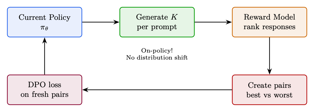
Figure 8.1: Approximate quality vs. compute frontier. Methods above the SFT ceiling line improve beyond what supervised fine-tuning alone achieves. Position is illustrative and model-dependent.

Decision Tree: Which Method to Use?

1. Do you have verifiable rewards? (math/code) →GRPO

2. Do you need max quality on complex tasks? →PPO

3. Do you have paired preferences? →DPO (or IPO if noisy)

4. Only unpaired binary feedback? →KTO

5. Memory-limited, starting from base model? →ORPO

6. DPO plateauing, want on-policy? →Online DPO

7. Need a strong baseline quickly? →Best-of-N / RFT

Chapter 9