System Architecture & Infrastructure at Scale
System Architecture & Infrastructure at Scale
System Architecture & Infrastructure at Scale
Training LLMs with reinforcement learning from human feedback is as much a systems engineering challenge as it is an algorithmic one. Unlike standard supervised fine-tuning--which involves a single model, a single forward-backward pass, and well-understood scaling--RLHF requires multiple models (policy, reference, reward model, value head) to be loaded simultaneously, coordinated through a complex rollout-scoring-training loop, and distributed across dozens to hundreds of GPUs. This chapter covers the systems-level details that make large-scale RLHF training possible: memory budgeting, parallelism strategies (Data, Tensor, Pipeline, Sequence, and their combinations), the generation bottleneck, decoupled architectures, weight synchronization, fault tolerance, and production monitoring.
11.1 The 4-Model Memory Challenge
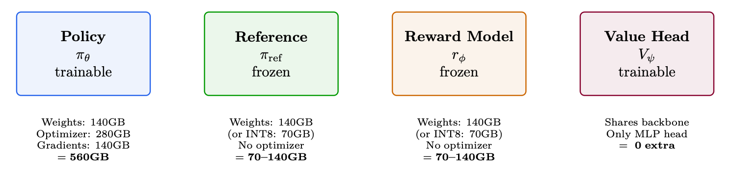
Figure 11.1: 70B PPO memory budget: the four models required for RLHF and their memory footprints. Total: 1470-1560GB. Minimum 19-20 A100-80GB (naive). With ZeRO-3: fits in 8 nodes.
Memory Budget Reality Check - 70B BF16
Policy weights (BF16) 140 GB
FP32 master weights 280 GB Adam optimizer (m + v, FP32) 560 GB Gradients (BF16) 140 GB Reference model 140 GB (or 70 GB in INT8) Reward model 140 GB (or 70 GB in INT8) Activations (batch 128, seq 2048) 50-100 GB KV cache for generation 20-60 GB Total 1470-1560 GB
÷ 80 GB/GPU = 19-20 A100s minimum (without any parallelism overhead).
Training large language models requires distributing computation across many GPUs. There are fundamentally different axes along which to parallelize, each with distinct trade-offs. This section provides detailed coverage of each strategy with mathematical formulations, diagrams, and practical guidance.
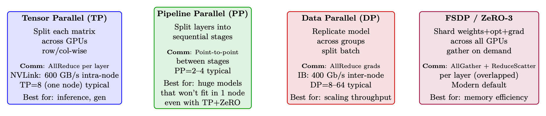
Figure 11.2: Overview of the four parallelism strategies. Production systems typically combine 2-3 of these simultaneously.
11.2.1 Data Parallelism (DP) and Distributed Data Parallelism (DDP)
Data Parallelism is the simplest and most common form of distributed training [205]. Each GPU holds a complete copy of the model, processes a different mini-batch, and synchronizes gradients.
Vanilla DP (PyTorch DataParallel). A single-process approach where one "master" GPU scatters input, gathers outputs, and broadcasts gradients. Limited by GIL and PCIe bandwidth to the master GPU.
Distributed Data Parallelism (DDP, DistributedDataParallel). Multi-process: each GPU runs its own process. Gradients are synchronized via ring-AllReduce [206] in the background while backward computation continues.
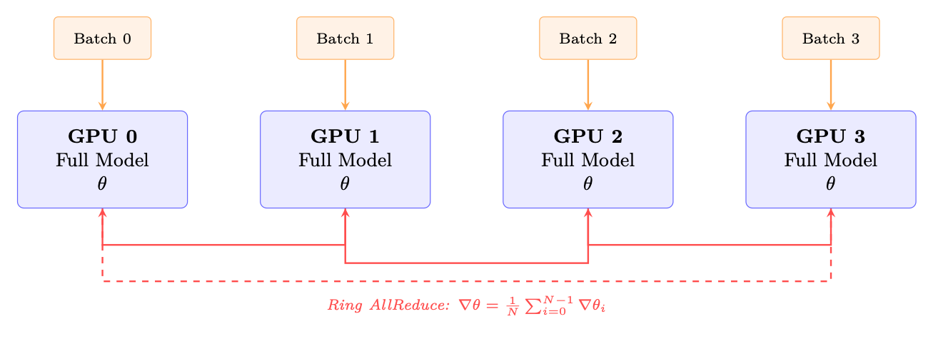
Figure 11.3: DDP: each GPU holds a full model replica and processes a different batch. Gradients are averaged via ring AllReduce, overlapped with backward computation.
Key properties of DDP:
• Memory: Each GPU stores full model + optimizer + gradients. For 70B BF16: ∼560 GB/GPU-- impossible without memory optimizations.
• Communication: One AllReduce of gradient tensor per step. Size = model parameters × 2 bytes (BF16). Ring AllReduce cost: 2 · N−1
N · M bytes transferred per GPU.
• Scaling: Near-linear up to ∼64 GPUs. Beyond that, communication starts to dominate.
• Gradient bucketing: DDP groups parameters into buckets (default 25 MB) and starts AllReduce as soon as a bucket's gradients are ready--overlapping communication with backward computation.
import torch.distributed as dist from torch.nn.parallel import DistributedDataParallel as DDP
dist. init_process_group (backend="nccl") # NCCL for GPU communication model = model.to(local_rank) model = DDP(model , device_ids =[ local_rank],
gradient_as_bucket_view =True , # Memory optimization static_graph=True) # Enable comm optimizations
DP vs DDP -- Always Use DDP
PyTorch's legacy DataParallel (DP) should never be used for LLM training:
• Single-process, limited by Python GIL
• All gradients funnel through GPU 0 (bottleneck)
• 2-3× slower than DDP even on a single node
• Cannot scale beyond one machine
DDP is the minimum parallelism strategy. For LLMs >7B, FSDP/ZeRO is preferred.
11.2.2 Tensor Parallelism (TP)
Tensor Parallelism (Megatron-LM style [207]) splits individual weight matrices across GPUs. Each GPU computes a partial result, and an AllReduce combines them.
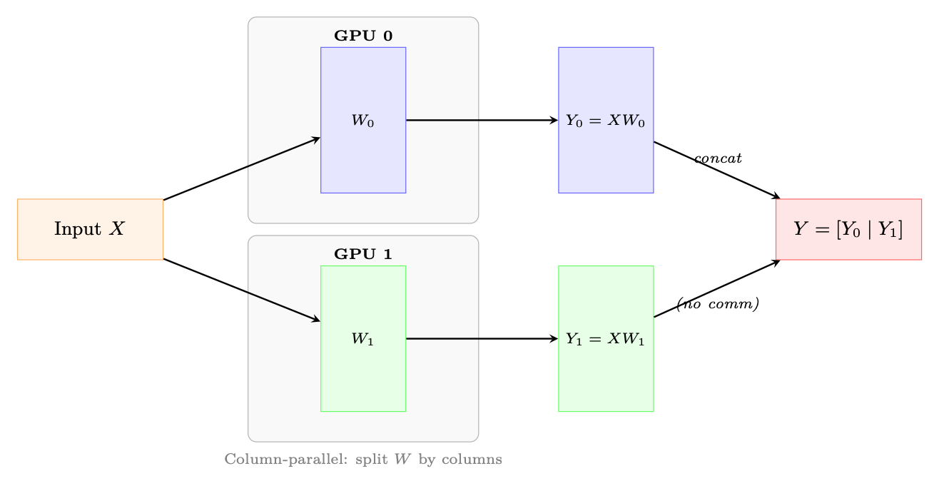
Column-Parallel Linear Layer. The weight matrix W ∈Rd×h is split column-wise across T GPUs: W = [W0 | W1 | · · · | WT−1], Wi ∈Rd×h/T (11.1)
Each GPU i computes Yi = XWi independently (no communication). The output is split along the hidden dimension.
Row-Parallel Linear Layer. The weight matrix is split row-wise: W = [W0; W1; . . . ; WT−1] where Wi ∈Rd/T×h. Input X must also be split. Each GPU computes a partial sum, then an AllReduce produces the final output.
1. MLP: Column-parallel for the first linear (h →4h), row-parallel for the second (4h →h). One AllReduce after the row-parallel layer.
2. Attention: Q, K, V projections are column-parallel (split heads across GPUs). Output projection is row-parallel. One AllReduce after output projection.
3. Total: 2 AllReduce per transformer layer (one for attention, one for MLP).
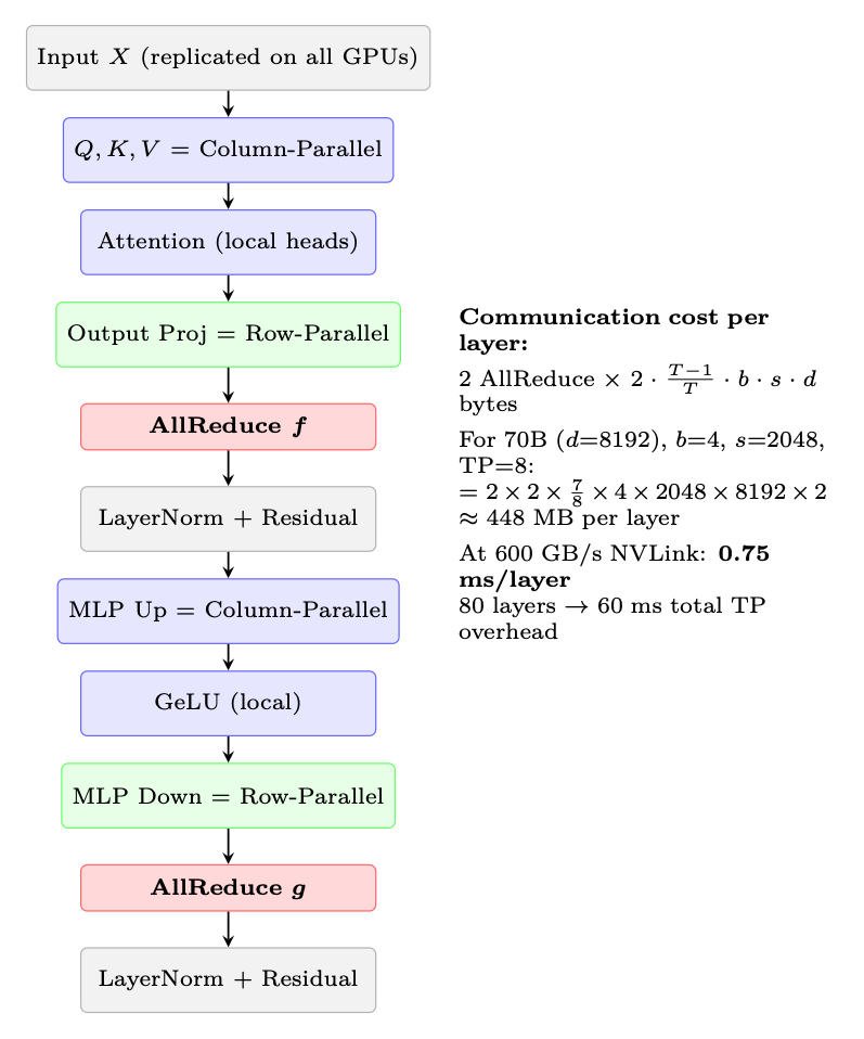
Figure 11.5: Tensor Parallel communication pattern in one Transformer block. Two AllReduce operations (marked in red) are required per layer--one after attention, one after MLP.
Why TP is Restricted to Intra-Node
Each transformer layer requires 2 AllReduce operations (marked as f and g above). For a 70B model with 80 layers, that's 160 AllReduce operations per forward pass (320 including backward). At NVLink speeds (600 GB/s), each AllReduce takes <0.5 ms. But over InfiniBand (50 GB/s), the same operation takes ∼4 ms, making the total overhead 160 × 4 = 640 ms--longer than the computation itself.
TP Degree Selection
• TP=1: No tensor parallelism. Model fits on one GPU (typically ≤13B with BF16).
• TP=2: Minimal split. Good for 13-34B inference on 2 GPUs. Low overhead (<5%).
• TP=4: Standard for 34-70B inference. Overhead 8-12%.
• TP=8: Full node. Required for 70B+ training. Overhead 12-18%.
• TP>8: Cross-node TP. Rarely used--only for 200B+ models where PP alone is insufficient. Overhead 30-50%.
Important: Number of attention heads must be divisible by TP degree. For LLaMA-70B (64 heads), valid TP = 1, 2, 4, 8, 16, 32, 64.
11.2.3 Sequence Parallelism (SP)
Sequence Parallelism [208] addresses a memory bottleneck that Tensor Parallelism alone cannot solve: the activation memory in LayerNorm and Dropout layers.
The Problem. With TP, weight memory is split across GPUs. But LayerNorm and Dropout operate on the full hidden dimension and are replicated on every GPU. Their activations (needed for backward pass) consume memory proportional to b × s × d--the same on every GPU, unreduced by TP.
The Solution. Split the sequence dimension for operations that don't require cross-GPU communication (LayerNorm, Dropout, residual connections). Each GPU processes a s/T slice of the sequence for these operations, then gathers the full sequence only where needed (attention, linear layers).
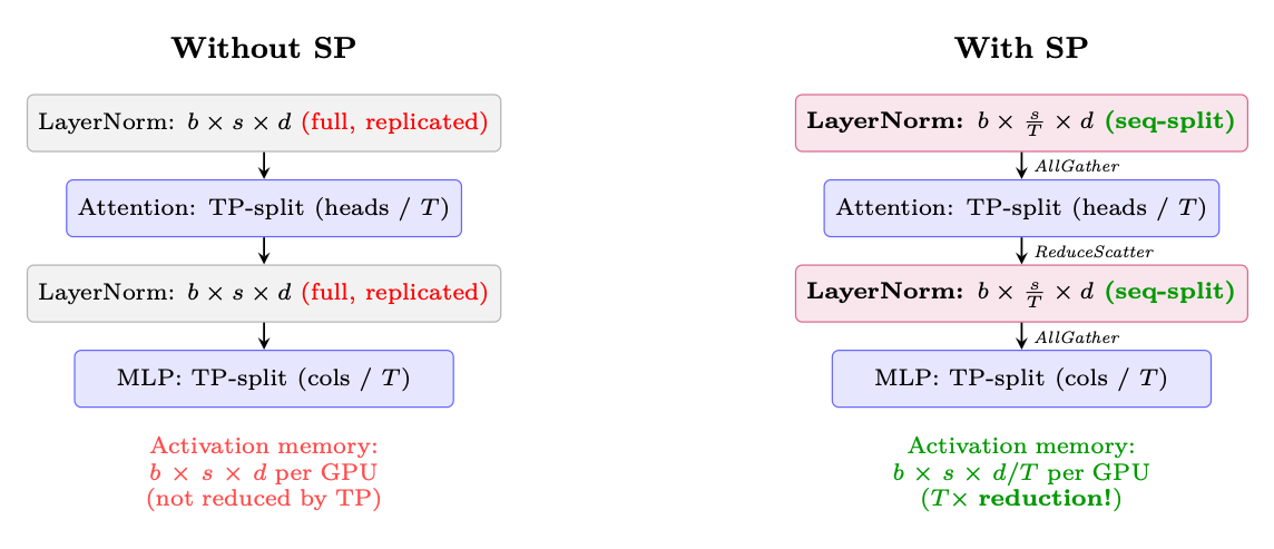
Figure 11.6: Sequence Parallelism reduces activation memory for LayerNorm/Dropout by splitting along the sequence dimension. Communication (AllGather/ReduceScatter) replaces the AllReduce used in standard TP--same total bytes transferred, but memory is saved.
SP Communication is "Free" Standard TP uses AllReduce after each sub-layer, which is equivalent to ReduceScatter + AllGather. SP simply reorders these primitives:
• TP without SP: AllReduce (= ReduceScatter + AllGather) →same data on all GPUs → LayerNorm on full tensor (wasteful).
• TP with SP: ReduceScatter →each GPU has 1/T of sequence →LayerNorm on partial tensor →AllGather before next TP layer.
Memory savings from SP (70B model, TP=8, batch=4, seq=2048):
Activation savings = (T −1)×b×s×d×nlayers×2 bytes = 7×4×2048×8192×80×2 ≈59 GB/GPU (11.2)
11.2.4 Pipeline Parallelism (PP)
Pipeline Parallelism splits the model vertically by layers, assigning consecutive groups of layers to different devices (stages). Activations flow forward through stages; gradients flow backward.
The Bubble Problem. Naive pipeline execution creates "bubbles"--idle time while a stage waits for input from the previous stage or gradients from the next:
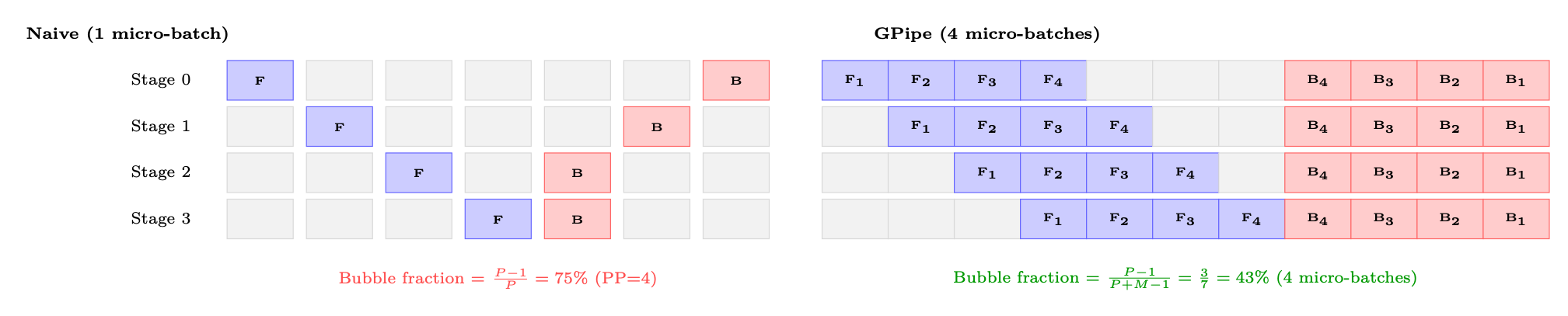
Figure 11.7: Pipeline bubble comparison. Left: naive pipeline with one micro-batch has 75% idle time. Right: GPipe with M = 4 micro-batches reduces bubbles significantly. With M ≫P, bubble fraction approaches zero.
Bubble Fraction Formula. For P pipeline stages and M micro-batches per step:
Bubble fraction = P −1 P + M −1 ≈P −1
M (when M ≫P) (11.3)
To keep bubble overhead <10%, you need M ≥10 · (P −1). For PP=4: at least 30 micro-batches.
Table 11.1: Pipeline scheduling strategies
Schedule Bubble Memory Characteristics
GPipe P−1 M+P−1 M× activations Simple; all-forward then allbackward [209] 1F1B P−1 M+P−1 P× activations Interleaved; steady-state memory bounded [210] Interleaved 1F1B P−1 M·V +P−1 P× activations Virtual stages (V ); further reduces bubble [211] Zero-Bubble (ZB-H1) ≈0 P× activations Splits backward into B and W phases [212]
Pipeline Schedules.
1F1B: The Production Standard The 1F1B (one-forward-one-backward) schedule [210] is used in most production systems (Megatron-LM [211], DeepSpeed [213]): Warmup: Forward passes fill the pipeline (P-1 micro-batches). Steady state: Alternate one forward and one backward per time slot. This bounds peak activation memory to P micro-batches (vs M for GPipe). Cooldown: Remaining backward passes drain the pipeline. Memory advantage: GPipe must store activations for all M micro-batches simultaneously. 1F1B only stores P sets of activations at steady state--critical when M = 32 but P = 4.
Data per transfer = bmicro × s × d × 2 bytes (BF16) (11.4)
For micro-batch=4, seq=2048, d=8192: 4 × 2048 × 8192 × 2 = 128 MB per transfer. At InfiniBand 50 GB/s: 2.6 ms per transfer--small relative to compute per stage.
Load Balancing. Not all layers have equal compute:
• Embedding layer: Very cheap (lookup table).
• Transformer blocks: Uniform compute.
• Final LM head: Moderate (large matrix multiply for vocabulary projection).
Assign more transformer layers to middle stages and fewer to the first/last stages to balance compute.
11.2.5 Fully Sharded Data Parallelism (FSDP / ZeRO-3)
FSDP [214] (PyTorch) and ZeRO-3 [213] (DeepSpeed) address the memory duplication inherent in DDP: instead of every GPU holding a full copy of parameters, gradients, and optimizer states, each GPU owns only a 1/N slice and reconstructs the full tensor on-the-fly when needed.
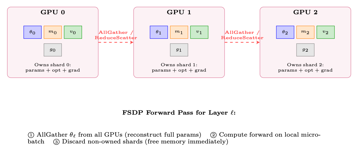
Figure 11.8: FSDP shards all model state across GPUs. Each GPU owns 1/N of parameters, optimizer states, and gradients. Full parameters are reconstructed on-demand via AllGather before each layer's computation.
FSDP execution flow per layer:
1. Forward: AllGather parameters →compute →discard non-owned shards.
2. Backward: AllGather parameters (again) →compute gradients →ReduceScatter gradients (each GPU gets its gradient shard) →discard non-owned parameter shards.
3. Optimizer step: Each GPU updates only its owned shard using its gradient shard and optimizer states.
Strategy Sharded Memory/GPU Communication
DDP (no sharding) Nothing 1120 GB × AllReduce (gradients only) ZeRO-1 Optimizer states 385 GB × AllReduce (gradients) ZeRO-2 Optimizer + gradients 368 GB × AllReduce (gradients)
ZeRO-3 / FSDP Everything 140 GB ✓ AllGather + ReduceScatter (per layer)
# Wrap model with FSDP auto_wrap = partial( transformer_auto_wrap_policy ,
transformer_layer_cls ={ LlamaDecoderLayer }) mp_policy = MixedPrecision(
param_dtype=torch.bfloat16 , reduce_dtype=torch.bfloat16 , buffer_dtype=torch.bfloat16 , )
model = FSDP(
model , sharding_strategy = ShardingStrategy .FULL_SHARD , # ZeRO -3 mixed_precision =mp_policy , auto_wrap_policy =auto_wrap , # Wrap each transformer layer use_orig_params =True , # Required for torch.compile compatibility limit_all_gathers =True , # Bound peak memory (1 AllGather in flight at a time)
forward_prefetch =True , # Prefetch next layer 's params during current layer
backward_prefetch = BackwardPrefetch .BACKWARD_PRE , # Prefetch during backward )
FSDP Communication Volume FSDP communicates 3× more data than DDP per step:
• DDP: 1 AllReduce of gradients = 2M bytes total across ring (where M = model size in bytes).
• FSDP: 2 AllGather (forward + backward) + 1 ReduceScatter = 3M bytes.
This is the memory-communication trade-off. FSDP is worthwhile when: (a) model doesn't fit in GPU memory with DDP, or (b) communication is well-overlapped with compute (modern frameworks achieve 70-90% overlap).
11.2.6 3D Parallelism: Combining Strategies
Production systems at scale (70B+) combine TP, PP, and DP/FSDP simultaneously:
Production Recipe: 70B on 64 A100-80GB (8 nodes)
Intra-node (NVLink 600GB/s): TP=8 for generation, FSDP within node for training.
Inter-node (InfiniBand 400Gb/s): FSDP across nodes (8-way data parallel).
Result: Each GPU holds ∼70GB. Policy weights gathered per-layer during forward/backward.
Pipeline Parallel: Only if model exceeds 100B+ and won't fit with TP+ZeRO. Adds complexity (bubble overhead 10-20%) and scheduling headaches.
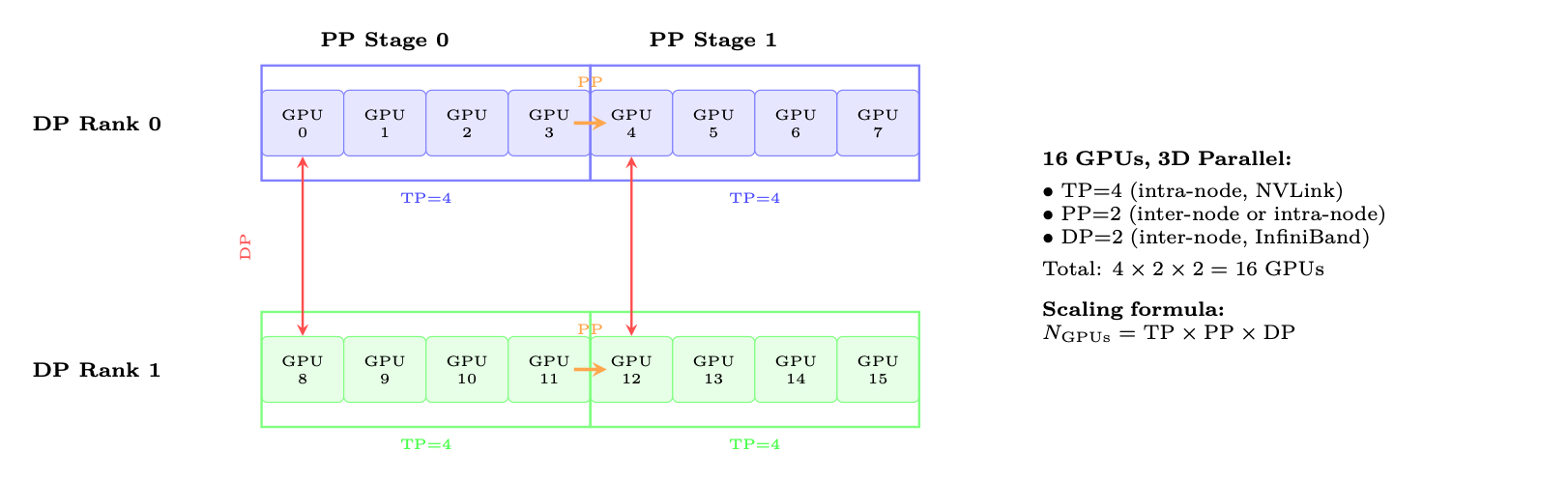
Figure 11.9: 3D parallelism layout for 16 GPUs: TP=4 (within each box, using NVLink), PP=2 (orange arrows, stages), DP=2 (red arrows, gradient sync). Each dimension exploits a different level of the communication hierarchy.
Decision flowchart:
1. Does the model fit on 1 GPU? →Use DDP.
2. Does it fit on 1 node with FSDP? →Use FSDP (ZeRO-3).
3. Does it fit on 1 node with TP+FSDP? →Use TP (intra-node) + FSDP (inter-node).
4. Still doesn't fit? →Add PP across nodes. This is the last resort.
Table 11.3: Parallelism strategy comparison summary
Strategy Splits Communication Scaling Limit Overhead When to Use
DP/DDP Batch AllReduce (grads) ∼64 GPUs 5-10% Model fits on 1 GPU FSDP Params+Opt+Grad AllGather+RS 100s of GPUs 10-20% Default for >13B TP Weight matrices AllReduce (2/layer) 8 GPUs (1 node) 12-18% Large model inference+train SP Activations (seq) Reuses TP comms Same as TP ≈0% extra Always with TP PP Layers (stages) Point-to-point ∼16 stages 15-30% 100B+ models only
11.3 The Generation Bottleneck: Quantitative Analysis
Roofline Analysis: Why Generation is Memory-Bound
A100 specs: 312 TFLOPS (BF16 tensor cores), 2 TB/s HBM bandwidth. Roofline crossover: 312T/2T = 156 FLOP/byte. Operations below 156 FLOP/byte are memory-bound. Autoregressive generation: For each token, read all weights (140GB for 70B) and do 2× 70B = 140G FLOPs per token (at batch=1). Arithmetic intensity: 140G FLOP/140GB = 1 FLOP/byte. That's 156× below the roofline! Utilization: 1/156 = 0.6% of peak FLOPS utilized. The GPU is 99.4% idle, waiting for memory reads. Token rate: 2TB/s/140GB = 14.3 tokens/second (single stream, batch=1). For 512 tokens: 512/14.3 = 35.8 seconds per response (batch=1, TP=1). Batching helps: Batch=64 with TP=4 →reads weights once, generates 64 tokens in parallel. Arithmetic intensity: 64 × 1 = 64 FLOP/byte. Better, but still below roofline!
Table 11.4: Generation throughput for 70B model (512 tokens, various configurations)
Config Batch Time/batch Tok/s/GPU Notes
1. vLLM + PagedAttention [157] (2-4×): Eliminates KV cache fragmentation, enables larger batches
2. Continuous batching [215] (1.5-2×): Don't wait for longest sequence; start new ones as others finish
3. Speculative decoding [143] (2-3×): Small draft model proposes 5 tokens, large model verifies in one forward pass. Accept 3-4 on average.
4. INT8/FP8 weights for gen (2×): Halve bandwidth needs. Quality loss is minimal since we're sampling (not computing exact logits for training)
5. CUDA graphs (1.1-1.3×): Eliminate kernel launch overhead for fixed-shape operations
6. Prefix caching (1.5× for shared-prefix prompts): Don't recompute system prompt KV cache
# Production vLLM generation setup from vllm import LLM , SamplingParams
engine = LLM(
model="./ policy_checkpoint ", tensor_parallel_size =4, # TP=4 per instance gpu_memory_utilization =0.92 , # Leave headroom for KV cache max_num_batched_tokens =16384 , # Max tokens in flight max_num_seqs =256, # Max concurrent sequences dtype="bfloat16", enable_prefix_caching =True , # Cache system prompt KV speculative_model ="./ draft_1B", # Speculative decoding num_speculative_tokens =5, block_size =16, # PagedAttention block size swap_space =4, # GB swap space for preemption )
# Generate responses for RLHF batch sampling_params = SamplingParams(
temperature =0.7, top_p =0.9, max_tokens =512 , logprobs =1, # Need log -probs for PPO ratio calculation ) outputs = engine.generate(prompts , sampling_params ) # Extract: responses , log_probs for each token (needed for PPO/GRPO)
11.4 Decoupled Architecture: Production Design
Production RLHF systems such as DeepSpeed-Chat [216] and OpenRLHF [217] use a decoupled architecture that separates generation, scoring, and training into independently scalable clusters.
Why Decouple?
Generation is memory-bandwidth bound (need fast HBM, waste compute).
Training is compute-bound (need tensor cores, waste bandwidth during backprop).
Same hardware can't optimize both: If you put everything together, you either waste compute during generation or waste bandwidth during training. Decoupling lets each cluster use optimal hardware/config. Practical benefits:
• Scale generation and training independently
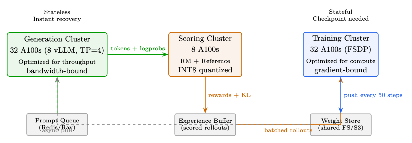
Figure 11.10: Decoupled RLHF architecture. Each cluster optimized for its workload. Scored rollouts accumulate in the experience buffer before being consumed by training.
• Generation cluster is stateless →trivial fault tolerance
• Can overlap gen(step N + 1) with training(step N) →30-40% speedup
• Different quantization: INT8 for generation (bandwidth), BF16 for training (precision)
11.5 Weight Synchronization Strategies
Strategy Staleness Bandwidth Quality Impact
Synchronous (every step) 0 steps 140 GB/step Perfect but too slow Periodic (every 50 steps) 25 avg 2.8 GB/step amortized <2% quality loss Delta compression (INT8) 25 avg 0.4 GB/step <3% quality loss Async streaming 5-10 steps 14 GB/step (background) <1% quality loss
Why Staleness is OK for PPO/GRPO
PPO's clipped objective was designed for off-policy data! The clip [1 −ϵ, 1 + ϵ] bounds the impact of stale data. With 10-50 steps of staleness:
• Policy changes ∼0.1-1% per step (with proper LR)
• Over 50 steps: ∼5% policy drift
• PPO clip handles up to 20% drift by design
• Empirically: quality loss <2% for 50-step staleness
Bandwidth math: 70B BF16 = 140GB. InfiniBand 400Gb/s = 50GB/s →full sync in 2.8s. With delta compression: <0.5s. Async = free (runs in background).
11.6 Memory Optimization Techniques
ZeRO Stage What Gets Sharded Memory/GPU (70B, 8 GPUs)
None (Data Parallel) Nothing (full replica) 560GB per GPU (impossible) ZeRO-1 Optimizer states only 175GB ZeRO-2 Optimizer states + Gradients 105GB ZeRO-3 (FSDP) Optimizer + Gradients + Parameters 70GB (fits in A100-80GB!)
Additional techniques:
• CPU offloading (ZeRO-Infinity [220]): Move optimizer states to CPU RAM. 50% memory savings but 2-3× slower (PCIe 64GB/s bottleneck).
• Activation offloading: Move activations to CPU during forward, bring back for backward. Only when memory is truly critical.
• Flash Attention [7, 82]: O(n) memory instead of O(n2) for attention. 2-4× faster + massive memory savings for long sequences.
11.6.1 Flash Attention's Impact on RLHF
Why Flash Attention Matters for RLHF
RLHF involves generating long sequences (rollouts) and then training on them. Without Flash Attention:
• A 4K-token sequence with 32 heads requires ∼4 GB just for attention matrices
• This severely limits batch size during PPO/GRPO training
• Gradient checkpointing of attention activations is expensive
With Flash Attention:
• Attention memory is O(n) - dominated by Q, K, V, O tensors
• Longer rollouts (8K-32K tokens) become feasible with the same GPU memory
• Backward pass recomputes attention tiles from Q, K, V (no stored n2 matrix)
• This is the key enabler for long-context RLHF (e.g., reasoning models)
Flash Attention and Gradient Checkpointing
Flash Attention's backward pass recomputes the attention tiles on-the-fly from Q, K, V (which are stored). This means Flash Attention already implements a form of activation recomputation for the O(n2) attention matrix. You do not need to additionally checkpoint the attention layer doing so would recompute Q, K, V unnecessarily.
# DeepSpeed ZeRO -3 configuration for 70B RLHF training ds_config = {
"bf16": {"enabled": True}, " zero_optimization ": {
"stage": 3, "overlap_comm": True , # Overlap communication with compute
" contiguous_gradients ": True , # Better memory layout " reduce_scatter": True , # More efficient than allreduce " reduce_bucket_size ": 5e7 , # 50M params per bucket " prefetch_bucket_size ": 5e7 , # Prefetch next bucket " param_persistence_threshold ": 1e5 , # Keep small params on all GPUs " offload_optimizer ": {"device": "cpu", "pin_memory": True}, # CPU offload " sub_group_size": 1e9 , # Reduce fragmentation }, " gradient_accumulation_steps ": 4, " gradient_clipping ": 1.0, " train_micro_batch_size_per_gpu ": 2, " wall_clock_breakdown ": True , }
Hardware Failure Reality
Individual GPU MTBF: ∼10,000 hours. 512-GPU cluster MTBF: 10000/512 ≈20 hours. But with software/network: 4-8 hours realistically. Multi-day training run: Will see 5-15 failures. Without fault tolerance, one failure kills everything.
Production fault tolerance stack:
1. Detection: NCCL timeout (60s), GPU heartbeat (10s), NVML health monitoring, ECC error counting.
2. Checkpointing: Async every 50-100 steps. Non-blocking (background thread). Save: model weights, optimizer states (Adam m/v), scheduler state, RNG states, KL coefficient, replay buffer. Keep last 3 checkpoints. Time: ∼30s for 70B (parallel write to NVMe).
3. Recovery: (a) Generation cluster = stateless, just restart and load latest weights. (b) Training cluster: load checkpoint, rebuild NCCL process group excluding failed node, redistribute FSDP shards, resume from last checkpoint.
4. Elastic training: Torch Elastic / Kubernetes auto-scaling. Replace failed node within minutes. Training continues with N −1 GPUs temporarily.
5. Prevention: GPU health pre-screening (run GEMM stress test before starting). Hot spares on standby. Redundant network paths (dual-rail InfiniBand).
11.8 End-to-End Latency Breakdown
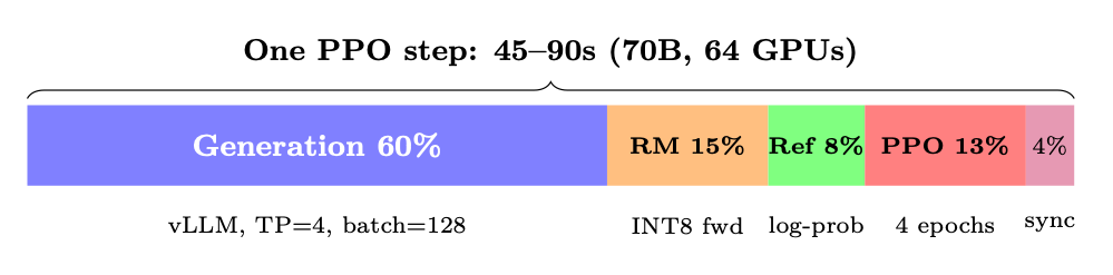
Figure 11.11: Without overlap (monolithic). With decoupled: gen overlaps with training, effective 1.4× speedup.
Phase Time (70B) Bound By Optimization
Generation (128×512 tok) 30-45s Memory bandwidth vLLM, spec decoding, INT Reward scoring 5-8s Compute (batch forward) INT8 RM, batch=128
Reference log-probs 4-6s Compute (batch forward) INT8 ref, or LoRA (free)
Key Metrics to Track During RLHF Training
Quality metrics (log every 10 steps):
• Mean reward (should increase then plateau)
• KL divergence from reference (should stay 3-10)
• Response length distribution (watch for length hacking)
• Entropy (should decrease slowly, not collapse)
System metrics (log every step):
• GPU utilization (target: >80% during training, >60% during gen)
• Memory watermark per GPU (catch OOM before it happens)
• Generation throughput (tokens/sec, should be stable)
• Gradient norm (spikes = instability incoming)
• NCCL communication time (detect network degradation)
11.10 Network Topology and Communication Patterns
Efficient distributed training requires understanding the hierarchical communication fabric that connects GPUs. Modern clusters use a two-tier architecture: ultra-fast intra-node links and slower but scalable inter-node networks.
11.10.1 Intra-Node: NVLink and NVSwitch
Table 11.5: NVLink generations and their impact on LLM training
Generation BW per link Links/GPU Total BW Platform
NVLink 3.0 50 GB/s 12 600 GB/s A100 (DGX A100) NVLink 4.0 50 GB/s 18 900 GB/s H100 (DGX H100) NVLink 5.0 100 GB/s 18 1800 GB/s B200 (DGX B200)
Within a single node (typically 8 GPUs), NVSwitch provides full-bisection bandwidth between all GPU pairs. This means any GPU can communicate with any other at full NVLink speed simultaneously--critical for Tensor Parallelism where every layer requires an AllReduce across all 8 GPUs.
NVSwitch vs PCIe Topology
With NVSwitch (DGX/HGX): All 8 GPUs connected all-to-all at 600-1800 GB/s. AllReduce for TP takes ∼0.2ms per layer. Without NVSwitch (PCIe-only servers): GPUs communicate through CPU PCIe root complex at 32-64 GB/s. TP across 8 GPUs becomes 10-30× slower. Never use TP>2 on PCIe-only systems.
11.10.2 Inter-Node: InfiniBand and RoCE
Technology Bandwidth Latency Notes
InfiniBand NDR 400 Gb/s (50 GB/s) 1-2 µs Gold standard, RDMA, lossless InfiniBand NDR (dual-rail) 800 Gb/s (100 GB/s) 1-2 µs Used in H100 clusters RoCE v2 100-400 Gb/s 2-5 µs Cheaper, needs PFC/ECN tuning Ethernet (TCP) 100-400 Gb/s 10-50 µs Not suitable for >16 GPU training
11.10.3 Communication Primitives and Their Costs
Understanding when each collective is used helps diagnose bottlenecks:
Table 11.7: NCCL collective operations in distributed LLM training
Collective Data Moved Used By When
AllReduce 2 · N−1
N · M TP, DP Sum gradients or activations across GPUs AllGather N−1
N · M FSDP forward Reconstruct full parameter tensor before matmul ReduceScatter N−1
N · M FSDP backward Distribute gradient shards after backprop Broadcast M PP Send activations to next pipeline stage Send/Recv M PP Point-to-point between adjacent stages
where M is the message size (bytes) and N is the number of participants.
Modern frameworks (FSDP, DeepSpeed) aggressively overlap communication with computation: Forward pass: While layer i computes, AllGather prefetches parameters for layer i + 1. After layer i finishes, its parameters are immediately discarded ("free-after-forward"). Backward pass: While layer i computes gradients, ReduceScatter sends layer i + 1's gradients. This overlap hides 70-90% of communication latency when properly tuned. Tuning knobs: prefetch_factor (how many layers ahead to prefetch), reduce_bucket_size (granularity of gradient reduction), backward_prefetch ("pre" vs "post" backward prefetch strategy).
11.10.4 Network Topology Design
Production clusters use fat-tree or rail-optimized topologies:
• Fat-tree: Full bisection bandwidth at every level. Any node can communicate with any other at full speed. Expensive (many switches) but maximally flexible.
• Rail-optimized: GPU i on every node connects to the same leaf switch ("rail i"). AllReduce within a rail is cheap; cross-rail traffic is expensive. Used by Meta's RSC and Google's TPU pods.
• 3D torus / Dragonfly: Used in HPC clusters (Frontier, Aurora). Topology-aware job placement is critical.
Job Placement Matters On a 512-GPU cluster, random node assignment can cause 2-3× slowdown due to network congestion. Always request contiguous node blocks. Production schedulers (Slurm, Kubernetes) should enforce locality: all nodes in a training job should be on the same leaf switch or within one hop of each other.
11.11 Training Throughput and Model FLOPs Utilization
11.11.1 Measuring Training Efficiency: MFU
Model FLOPs Utilization (MFU) [221] is the standard metric for training efficiency:
MFU = Observed throughput (tokens/sec) × FLOPs per token
Peak hardware FLOPS (11.5)
For a transformer with P parameters, s sequence length, and b batch size:
FLOPs per token ≈6P + 12 · nlayers · dmodel · s (11.6)
The factor of 6 comes from: 2 (multiply-add) × 3 (forward + backward, where backward ≈2× forward). The second term accounts for attention's O(s2) cost.
Why MFU Decreases with Scale
Larger models require more parallelism, which introduces:
1. Communication overhead: AllGather/ReduceScatter for FSDP (∼10-15% at 64 GPUs)
2. Pipeline bubbles: PP introduces idle time at start/end of micro-batches (∼15-25% with PP=4)
3. Memory for auxiliary models: Reference/RM take GPU memory that could hold larger batches
4. Load imbalance: Not all layers have equal compute (embeddings vs transformer blocks)
Model Hardware MFU Tokens/sec/GPU Configuration
LLaMA-7B 8×A100 57% 3,200 FSDP, FlashAttn, BF16 LLaMA-13B 16×A100 52% 1,750 FSDP, FlashAttn, BF16 LLaMA-70B 64×A100 45% 380 FSDP+TP=8, FlashAttn GPT-4 (est.) 10,000+ H100 40-50% -- 3D parallelism PaLM-540B 6144 TPUv4 46% -- DP+TP+PP
Rule of thumb: Target MFU > 40% for training. If below 30%, diagnose with profiling.
11.11.2 Compute-Optimal Batch Sizing
The effective batch size interacts with hardware utilization in non-obvious ways:
Effective batch size = micro_batch × grad_accum × DP degree (11.7)
• Too small: GPU underutilized (low arithmetic intensity), communication dominates.
• Too large: Diminishing learning per token (critical batch size exceeded), wastes compute.
• Sweet spot: The critical batch size Bcrit where gradient noise equals gradient signal. For LLMs, Bcrit ∼1-4M tokens [222].
For RLHF specifically, the batch contains rollouts (not just tokens):
RLHF batch = Nprompts × Kgenerations × Lavg response length (11.8)
Typical production values: N = 128 prompts, K = 1-4 generations, L = 256-512 tokens → 32K-256K tokens per step.
11.11.3 Profiling and Bottleneck Diagnosis
Key profiling tools and what they reveal:
Tool Captures Best For
torch.profiler Kernel timing, memory Finding slow ops, memory leaks NVIDIA Nsight Systems Full GPU timeline Visualizing overlap, gaps between kernels nccl_debug=INFO Collective sizes/times Diagnosing communication bottlenecks torch.cuda.memory_stats Allocation patterns Finding fragmentation, peak usage DeepSpeed Flops Profiler Per-layer FLOPs Identifying load imbalance py-spy / scalene CPU profiling Data loading, tokenization bottlenecks
Diagnosing Low MFU: A Checklist
1. GPU utilization < 80%? →Data loading bottleneck (check CPU, I/O).
2. Large gaps between kernels? →Python overhead, synchronization points. Use CUDA graphs.
3. Communication > 20% of step time? →Reduce TP degree, increase batch size, check network health.
4. Memory at 99%? →Cannot increase batch. Try gradient checkpointing, offloading.
5. OOM during generation? →KV cache too large. Reduce max_seq_len or batch size for
11.12 Cost Analysis and Cloud Deployment
Understanding the economics of RLHF training is essential for planning.
11.12.1 Hardware Cost Comparison
Table 11.9: Approximate cloud GPU costs for RLHF training (2024-2025 pricing)
GPU On-Demand/hr Spot/hr Memory Use Case
A100 80GB $2.50-3.50 $1.00-1.50 80 GB HBM2e Budget training, gen cluster H100 80GB $4.00-6.00 $2.00-3.00 80 GB HBM3 Production training H200 141GB $6.00-8.00 -- 141 GB HBM3e Large context, fewerGPU configs MI300X 192GB $3.50-5.00 $1.50-2.50 192 GB HBM3 Cost-effective alternative
11.12.2 RLHF Training Cost Estimation
Cost = Nsteps × Tstep
3600 × NGPUs × CGPU/hr (11.9)
Cost Example: 70B Model RLHF (10K steps)
Steps 10,000
Time per step (decoupled) 45 seconds Total training time 10000 × 45/3600 = 125 hours GPUs (generation + training) 64 A100-80GB Cost per GPU-hour (spot) $1.20 Total cost 125 × 64 × $1.20 = $9,600 Breakdown by phase:
• Generation cluster (32 GPUs): $4,800 (60% of time)
• Training cluster (32 GPUs): $4,800 (could overlap →$3,400 effective)
• Scoring (shared with gen GPUs): included above
With overlap: Effective cost ≈$7,500 for full RLHF alignment of a 70B model.
11.12.3 Cost Optimization Strategies
• Spot/preemptible instances: 50-70% savings. Requires robust checkpointing (save every 5 minutes).
• Right-sizing: Don't use H100 for generation (memory-bound); A100 achieves similar tokens/$ for inference.
• Quantized inference: INT8/FP8 for generation and scoring halves GPU count for those clusters.
• Progressive training: Start with 8B proxy model for reward engineering/debugging (∼$200), then scale to 70B.
11.13 Distributed Checkpointing
At scale, naive checkpointing becomes a bottleneck. A 70B model with optimizer state requires saving ∼840 GB per checkpoint (FP32 master weights + Adam m + v).
11.13.1 Checkpointing Strategies
Table 11.10: Checkpointing approaches for large-scale RLHF
Strategy Save Time (70B) Storage/ckpt Characteristics
Synchronous (all ranks) 30-60s (blocking) 420 GB Simple, stalls training Async (background copy) <1s (non-blocking) 420 GB Overlaps with next step Incremental (delta) <1s 5-20 GB Only save changed params Sharded (FSDP native) 5-10s 420 GB sharded Each rank saves its shard
11.13.2 Production Checkpointing with torch.distributed.checkpoint
import torch.distributed.checkpoint as dcp from torch.distributed.checkpoint.state_dict import get_state_dict , StateDictOptions
# Save: each rank writes its shard in parallel state_dict = {"model": get_state_dict (model , options= StateDictOptions (
full_state_dict =False))} dcp.save(
state_dict=state_dict , storage_writer =dcp. FileSystemWriter ("/mnt/checkpoints/step_5000"), planner=dcp. DefaultSavePlanner (), # Handles FSDP sharding automatically )
# Async save: non -blocking , runs in background thread future = dcp.async_save(
state_dict=state_dict , storage_writer =dcp. FileSystemWriter ("/mnt/checkpoints/step_5000"), ) # Training continues immediately; future.result () blocks only if needed
Checkpoint Hygiene for RLHF
RLHF checkpoints must capture more than standard pre-training:
• Policy model weights + optimizer states (standard)
• KL coefficient (β) and its schedule state
• Replay buffer contents (for off-policy corrections)
• RNG states for all GPUs (reproducibility)
• Prompt iterator position (avoid re-processing prompts)
• Reward model version tag (for auditability)
• Wandb/metrics run ID (for continuous logging)
Choosing the right hardware depends on model size, budget, and training phase.
Table 11.11: Hardware recommendations by model scale and training phase
Model Size Training Phase Recommended Configuration
≤7B SFT + RLHF 1-2× A100 Single node, no parallelism needed 7-13B SFT + RLHF 4-8× A100 FSDP, optional TP=2 for gen 13-34B SFT + RLHF 8-16× A100/H100 FSDP + TP=4 for gen 70B RLHF (full) 32-64× A100/H100 Decoupled, FSDP + TP=8 70B RLHF (LoRA) 8-16× A100/H100 No ref model, LoRA adapters >100B RLHF 128+× H100 3D parallelism (TP+PP+DP)
H100 vs A100: When is the Upgrade Worth It?
H100 provides:
• ∼1.6× peak FLOPS (989 vs 624 TFLOPS for BF16 with sparsity; 495 vs 312 without sparsity)
• ∼2× memory bandwidth (3.35 vs 2.0 TB/s)
• FP8 support (additional 2× for inference)
• NVLink 4.0 (900 vs 600 GB/s)
For training: ∼1.8-2.2× faster end-to-end (FP8 support and higher bandwidth amplify the raw FLOPS advantage). For generation: ∼1.7× faster (bandwidth-bound, so 2× BW ≈1.7× throughput with overhead). Cost-performance: At 1.5× the price, H100 is almost always better value for training. For inference-only (generation clusters), A100 at spot pricing can be more cost-effective.
11.15 Optimizer Configuration for RL Training
RL training (PPO, GRPO, DPO) imposes unique demands on the optimizer compared to pretraining or SFT. The loss landscape is non-stationary (the policy changes what data is generated), gradients are noisier (reward signal variance), and training is more prone to catastrophic forgetting or reward hacking. This section consolidates RL-specific optimizer guidance, using AdamW [80] as the default optimizer.
11.15.1 Why RL Requires Different Optimizer Settings
RL vs. SFT Optimization - Key Differences
• Non-stationary data distribution: unlike SFT where the dataset is fixed, RL generates new rollouts each iteration--the data distribution shifts with the policy.
• High gradient variance: reward signals are sparse and noisy; gradients have much higher variance than cross-entropy on curated data.
• Smaller updates required: the policy must stay close to the reference model (KL constraint), so learning rates are 10-100× smaller than SFT.
• No weight decay: regularization comes from the KL penalty, not weight decay. Adding WD on top can fight the KL constraint.
• Shorter warmup: RL starts from a converged SFT checkpoint--the optimizer state needs minimal warmup.
Table 11.12: Optimizer settings for RL training phases. All use β1 = 0.9, β2 = 0.95, ϵ = 10−8, max_grad_norm=1.0, BF16.
Method Optimizer LR WD Warmup Schedule
DPO AdamW 5e-7 0.0 50 steps Constant or Linear PPO (policy) AdamW 1e-6 0.0 20 steps Constant PPO (critic) AdamW 1e-6 0.0 20 steps Constant GRPO AdamW 1e-6 0.0 20 steps Constant
Why Constant Schedule for RL?
Cosine and linear-decay schedules assume a fixed training horizon and monotonically decreasing loss. RL training has neither: reward may plateau, spike, or oscillate unpredictably. A constant LR (after brief warmup) keeps the optimizer responsive throughout training. If you must decay, use a very gentle linear schedule with a high minimum LR ratio (≥0.5).
11.15.3 Beta-2 = 0.95 for RL: Faster Adaptation
The default Adam β2 = 0.999 gives a very long memory for the second moment (∼1000-step effective window). In RL training, the loss landscape changes rapidly as the policy evolves--the gradient variance from 1000 steps ago is irrelevant. Using β2 = 0.95 shortens the window to ∼20 steps, making the adaptive learning rate respond quickly to changing gradient statistics.
When beta2 = 0.95 Hurts
For very small batch sizes (e.g., batch=1 in online RL), β2 = 0.95 can make the second moment estimates too noisy. In this regime, use β2 = 0.99 as a compromise, or increase the effective batch size via gradient accumulation.
11.15.4 Mixed Precision for RL: FP32 Master Weights Are Critical
RL training is particularly sensitive to numerical precision:
• Gradients are noisier--small updates must accumulate accurately over many steps
• Learning rates are very small (10−6-10−7), making ∆θ ≪θ
• BF16 mantissa (7 bits ≈0.8% relative precision) cannot represent updates of magnitude 10−6
relative to weights of magnitude 100
Always use FP32 master weights for RL training. BF16-only training (no FP32 copy) reliably causes reward collapse in PPO/GRPO after 100-500 steps.
11.15.5 Gradient Clipping is Critical for RL
In PPO and GRPO, the reward signal can be highly variable, especially early in training. A single bad batch can produce gradients with norm > 100, which would completely destroy the model weights. max_grad_norm=1.0 is the standard setting. For SFT, clipping is less critical but still recommended.
Never Disable Gradient Clipping for RL
Unlike SFT where gradient norms are typically stable (0.1-1.0 range), RL gradients are spiky because: (1) reward variance propagates through the policy gradient, (2) rare high-reward trajectories create outsized updates, and (3) the KL penalty term can produce large gradients when the policy drifts. A single unclipped step with ∥∇∥> 50 can undo hundreds of training steps.
Red Flags and Fixes for RL Optimization
Symptom Likely Cause and Fix
Reward improves then collapses LR too high or KL coefficient too low. Reduce LR by 2-5× or increase βKL. Gradient norm constantly at clip threshold Updates too aggressive. Reduce LR (clipping means you're losing gradient direction info every step). KL divergence explodes (>15 nats) LR too high. Reduce by 10× or add adaptive KL penalty. Reward stuck at baseline LR too low, or reward model has low signal. Try 2-5× higher LR. Check reward model calibration. Loss NaN after 100+ steps FP32 master weights missing, or grad norm overflow. Enable FP32 master weights; verify BF16 mode.
11.15.7 HuggingFace TRL Configuration for RL
The TRL library [176] provides production-ready implementations of PPO, DPO, and other RL methods for LLMs.
from trl import PPOConfig , PPOTrainer , DPOConfig , DPOTrainer
# --- PPO Configuration --- ppo_config = PPOConfig(
# Optimizer (AdamW with RL -specific settings) learning_rate =1e-6, # 10 -100x smaller than SFT
# PPO -specific ppo_epochs =4, # mini -batch updates per rollout mini_batch_size =16, batch_size =64, # rollout batch size
# Gradient control max_grad_norm =1.0,
# KL penalty (replaces weight decay as regularizer) init_kl_coef =0.2, # initial KL penalty coefficient adap_kl_ctrl=True , # adaptive KL targeting target_kl =6.0, # target KL divergence
# Mixed precision bf16=True , # BF16 compute , FP32 master weights )
ppo_trainer = PPOTrainer(
model=model , ref_model=ref_model , config=ppo_config , tokenizer=tokenizer , dataset=dataset , )
# --- DPO Configuration --- dpo_config = DPOConfig(
output_dir="./ dpo_output",
# Optimizer learning_rate =5e-7, # even smaller than PPO optim="adamw_torch", adam_beta1 =0.9, adam_beta2 =0.95 , # shorter memory for RL weight_decay =0.0, # no WD -- KL provides regularization
# Gradient control max_grad_norm =1.0,
# DPO -specific beta =0.1, # KL constraint strength loss_type="sigmoid", # standard DPO loss
# Mixed precision bf16=True ,
# Training num_train_epochs =1, # DPO typically 1 epoch per_device_train_batch_size =4, gradient_accumulation_steps =8, )
dpo_trainer = DPOTrainer(
model=model , ref_model=ref_model , args=dpo_config , train_dataset=dataset , tokenizer=tokenizer , ) dpo_trainer.train ()
Listing 11.1: Complete PPO and DPO optimizer configuration using TRL.
11.15.8 MoE Considerations for RL Training
MoE for RLHF Mixture-of-Experts (MoE) models [109] are increasingly used in RLHF:
• Advantage: 3-4× more capacity at same compute cost. Better for reward models (more capacity to judge).
• Challenge: Expert parallelism requires all-to-all communication (tokens routed across GPUs). This conflicts with pipeline parallelism.
• GRPO with MoE: Works well since generation cost is dominated by active params (not total params).
• LoRA for MoE: Can apply LoRA to router + shared layers only, or to all experts (expensive).
The RL Optimizer Mantra
For RL fine-tuning: small LR, no weight decay, constant schedule, FP32 master weights, aggressive clipping. Let the KL penalty handle regularization--the optimizer's job is just to follow the policy gradient without overshooting.
Chapter 12